Example 1.1
We first import the packages used in this tutorial.
# Import libraries
library(mia)
library(ComplexHeatmap)
We also import Tengeler2020 from the mia package and store it into a variable.
# Load dataset and store it into tse
data("Tengeler2020", package = "mia")
tse <- Tengeler2020
Next, we transform the counts assay to relative abundance assay and store it into the TreeSE.
# Transform counts to relative abundances
tse <- transformAssay(tse, method = "relabundance")
Then, we agglomerate the experiment to the order level, so that information is more condensed and therefore easier to visualise and interpret.
# Agglomerate by order
tse_order <- agglomerateByRank(tse, rank = "Order")
Why relative abundances?
Microbiome data is compositional. Relative abundance helps us draw less biased comparisons between samples.
Show code
# Import packages
library(miaViz)
library(patchwork)

# Plot composition by counts
counts_bar <- plotAbundance(tse_order, rank = "Phylum", use_relative = FALSE) +
  ylab("Counts")

# Plot composition by relative abundance
relab_bar <- plotAbundance(tse_order, rank = "Phylum", use_relative = TRUE) +
  ylab("Relative Abundance")

# Combine plots
(counts_bar | relab_bar) +
  plot_layout(guides = "collect")
![]()
Figure 1: Sample composition by counts (left) or relative abundance (right).
Example 1.2
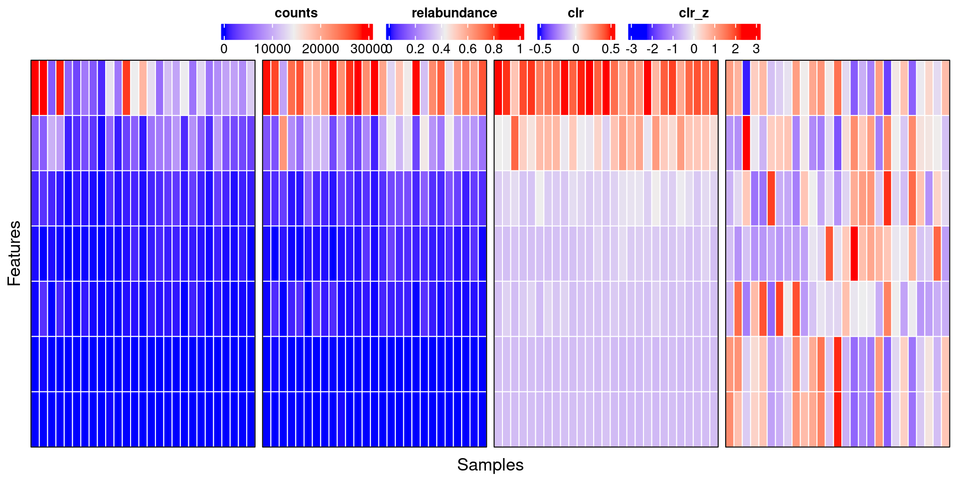
To reduce data skewness, we further transform the relative abundance assay with the Centered-Log Ratio (CLR), which is defined as follows:
\[
clr = log \frac{x}{g(x)} = log(x)−log[g(x)]
\]
where x is a feature and g(x) is the geometric mean of all features in a sample.
# Transform relative abundances to clr
tse_order <- transformAssay(tse_order,
                            assay.type = "relabundance",
                            method = "clr",
                            pseudocount = 1,
                            MARGIN = "samples")
Lastly, we get the row-wise z-scores of every feature from the clr assay to standardise abundances across samples.
# Transform clr to z
tse_order <- transformAssay(tse_order,
                            assay.type = "clr",
                            method = "z",
                            name = "clr_z",
                            MARGIN = "features")
Example 1.3
Finally, we visualise the clr-z assay with ComplexHeatmap.
# Visualise clr-z assay with a heatmap
clrz_hm <- Heatmap(assay(tse_order, "clr_z"), name = "clr-z")
clrz_hm
![]()
Figure 2: Heatmap of CLR-Z assay where columns correspond to samples and rows to taxa agglomerated by order.