Multivariate analysis

Multiple variables
Different methods
- Ordination-based methods
- Clustering
- Classification, …

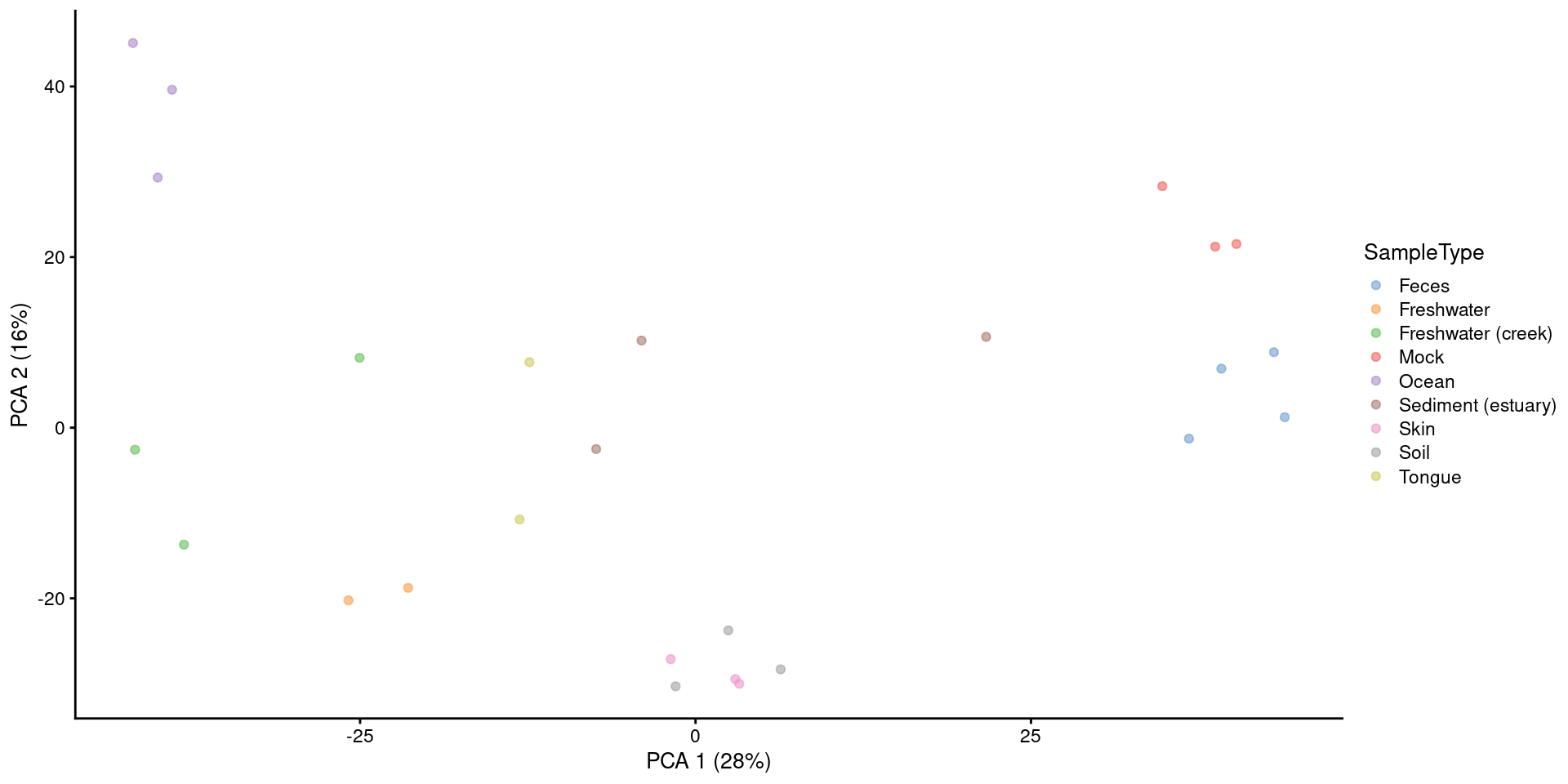
Ordination

Beta diversity: diversity between microbial communities
Simplify and visualize high-dimensional data
Projects data into lower dimensional latent space

Matrix factorization

Decomposes complex data into components
Widely used and general technique
Methods vary based on goals and constraints

Ordination methods

Different methods
- PCA, PCoA/MDS, RDA, …
Euclidean/non-Euclidean
Unsupervised/supervised

Principal component analysis (PCA)

Goal: Maximize the variance
Euclidean distance
Aitchison distance: CLR + Euclidean distance

Example 1.1: PCA

First we load an example dataset and apply robust clr transformation.

Show code

library(mia)
data("Tengeler2020")
tse <- Tengeler2020
# Transform data
tse <- transformAssay(tse, method = "rclr")

Then we perform PCA with runPCA()function available in scater package.

Show code

library(scater)

tse <- runPCA(
    tse,
    assay.type = "rclr"
    )

We can retrieve a list of all reduced dimensions with reducedDims().

Show code

reducedDims(tse)

List of length 1
names(1): PCA

If you need only their names, these can be accessed with reducedDimNames().

Show code

reducedDimNames(tse)

[1] "PCA"

And the results can be accessed with reducedDim(tse, "PCA").

Show code

reducedDim(tse, "PCA") |> head()

            PC1       PC2         PC3        PC4        PC5        PC6
A110 -4.5035339 -2.456547 -2.11328100 -3.8634688  2.0123949 -0.3325532
A12   2.4156363  4.982008 -0.07545471  0.1898264 -1.3925704  1.2237517
A15  -2.7404749 -3.121391 -4.46833577  8.1698047 -2.5837119 -2.1243919
A19   0.7358807  7.090486 -1.00797353 -1.2989823  0.1064523 -3.3824751
A21   0.4648846  5.448022 -1.14685965 -0.8743427  1.2143298 -4.4323282
A23  -2.0686346 -1.954092 -2.61287624 -2.5249816 -3.0007937 -2.4024629
            PC7        PC8        PC9       PC10         PC11       PC12
A110 -0.8342411  1.0193914 -4.2216208  1.1932256  0.172707622 -2.3565927
A12  -0.3055218  0.7968376  0.4988079  2.7782003  0.551278116  0.4895880
A15  -1.3546507  1.5617929 -0.7468926 -0.7977925 -0.002285458 -1.9595096
A19   1.4979577  0.1788277 -0.9825262 -2.3851223 -2.018251650 -1.4132247
A21   1.6593740  0.5619416  0.6748281 -0.2531164 -1.974152848  0.7930157
A23  -2.5300350 -3.0190698  3.9427392  0.2632914  1.180388830  0.3831161
           PC13       PC14       PC15        PC16       PC17       PC18
A110  0.2449630 -1.2664497  1.4364113  0.89583856  0.8365374  0.4457789
A12  -1.4948351 -2.5473097 -0.8648291 -1.48252017 -0.7839398  0.1476567
A15   0.4154040 -0.2455156  0.1621916  0.33095787 -0.7875945 -0.0824129
A19   0.1953649  0.9069244  0.2419303  0.38847386  1.4955734  0.3421782
A21  -1.2728108  0.7827710 -0.8452163 -0.58884502 -1.9694914 -0.5016079
A23  -0.8302655 -0.2890572  2.1834383  0.09925442  0.3728412 -1.4058642
             PC19       PC20       PC21       PC22       PC23       PC24
A110  0.987010794 -1.0053150 -0.9899730  0.8829111 -0.2200736 -0.2975089
A12   0.114383997  0.5743782 -1.9702511 -0.4000117 -0.2989457 -1.0332134
A15  -0.517904963  0.1558602 -0.2901768 -0.1773831 -0.4550756 -0.1875868
A19   0.480395457  1.3345829  0.8691778 -0.5697885  0.2015948 -0.7871444
A21   0.006978105 -1.8347856 -0.6948813  0.4662380 -0.3698014  0.5050710
A23   0.516079026 -0.8406535  0.3192697  0.3128884 -0.1924474 -0.2425484
            PC25        PC26
A110 -0.60890560 -0.20643929
A12   0.51342549 -1.06913557
A15  -0.04222125  0.01149364
A19   1.10441000 -0.77053190
A21  -1.05782664  0.59576805
A23   0.74942196 -0.01116033

Example 1.2: Visualize PCA

PCA or other ordination results are usually visualized with scatter plot.

Show code

plotReducedDim(
    tse,
    dimred = "PCA",
    colour_by = "patient_status"
    )

Example 1.3: PCA contributors

Some taxa contribute more than others to the generation of reduced dimensions.

Show code

library(miaViz)
plotLoadings(tse, "PCA", ncomponents = 2)

Exercises 1: PCA

29.7.1 Reduced dimensions retrieval
29.7.2 Visualization basics with PCA

Principal coordinate analysis (PCoA)

Goal: Preserve the dissimilarity structure
Non-Euclidean
Different dissimilarity metrics

When Euclidean distance is used, PCoA reduces to PCA.

Example 2.1: PCoA

We transform the counts assay to relative abundances and store the new assay back into the TreeSE.

Show code

# Transform counts to relative abundance
tse <- transformAssay(tse, method = "relabundance")

Here, we run PCoA on the relative abundance assay to reduce the dimensionality of the data. We set method to Bray-Curtis dissimilarity.

Show code

# Run PCoA with Bray-Curtis dissimilarity
tse <- runMDS(
    tse,
    assay.type = "relabundance",
    FUN = getDissimilarity,
    method = "bray"
    )

We can see that now there are additional results in reducedDim.

Show code

reducedDimNames(tse)

[1] "PCA" "MDS"

Example 2.2: Visualize PCoA

Similarly to PCA, we can visualize PCoA with scatter plot.

Show code

plotReducedDim(
    tse,
    dimred = "MDS",
    colour_by = "patient_status"
    )

Example 2.3: PCoA contributors

Loadings of PCoA cannot be interpreted as directly as PCA: “features that contribute the most to dissimilarity”.

Instead, we can calculate correlation between abundances and coordinates.

Show code

# Compute correlation between features and reduced dimensions
comp_loads <- apply(
    assay(tse, "relabundance"),
    MARGIN = 1, simplify = FALSE,
    function(x) cor(x, reducedDim(tse, "MDS"), method = "kendall")
)

# Prepare matrix of feature loadings
taxa_loads <- do.call(rbind, comp_loads)
colnames(taxa_loads) <- paste0("MDS", seq(ncol(taxa_loads)))
rownames(taxa_loads) <- rownames(tse)

The top PCoA loadings for the first two dimensions are visualised below.

Show code

plotLoadings(taxa_loads, ncomponents = 2)

Exercises 2: PCoA

29.7.3 Principal Coordinate Analysis (PCoA)

Redundancy analysis (RDA)

Supervised
How much covariate explains the differences in microbial profile?
Two steps
1. Principal Coordinate Analysis (PCoA)
2. Maximizes the variance explained by covariates

Example 2.1: dbRDA

We can apply dbRDA with runRDA() function. formula tells how the method is applied; here “patient_status” and cohort are the explanatory variables.

Show code

# Run PCoA with Bray-Curtis dissimilarity
tse <- addRDA(
    tse,
    formula = x ~ patient_status + cohort,
    assay.type = "relabundance",
    method = "bray"
    )

Example 2.2.: Visualize dbRDA

We can visualize dbRDA results with plotReducedDim() or plotRDA() which have additional features.

Show code

plotRDA(
    tse,
    dimred = "RDA",
    colour_by = "patient_status"
    )

Exercises 3: dbRDA

29.7.5 Redundancy analysis (RDA)
29.7.6 Beta diversity analysis

Extra:

Find the top 5 contributor taxa for principal component 1.

Example 3.1: Other Distances

A different distance function can be specified with FUN, such as phylogenetic distance.

Show code

# Run PCoA with Unifrac distance
tse <- runMDS(
    tse,
    assay.type = "counts",
    FUN = getDissimilarity,
    method = "unifrac",
    tree = rowTree(tse),
    ncomponents = 3,
    name = "Unifrac")

The number of dimensions to visualise can also be adjusted with ncomponents.

Show code

# Visualise Unifrac distance between samples
plotReducedDim(
    tse,
    "Unifrac",
    ncomponents = 3,
    colour_by = "patient_status"
    )

Example 3.2: Comparison

Different ordination methods return considerably different results, which can be compared to achieve a better understanding of the data.

Show code

library(patchwork)

# Generate plots for 
plots <- lapply(reducedDimNames(tse), function(name){
    plotReducedDim(tse, name, colour_by = "patient_status")
})

# Generate multi-panel plot
wrap_plots(plots) +
  plot_layout(guides = "collect") +
  plot_annotation(tag_levels = "A")

Exercise 3

Run MDS on the CLR assay with Euclidean distance and compare the results with the previous PCoA and PCA.

Extra:

Make a plot with the first three dimensions, and a plot with the second and fourth dimensions.

Resources

OMA Chapter - Community Similarity