Alpha Diversity

Overview

This notebook guides you through a basic alpha diversity analysis, where you first estimate alpha diversity in terms of a few indices, plot them for the different study groups and compare the results for the different indices.

The following packages are needed to succesfully run the examples in this notebook:

• mia: tools for microbiome data analysis

• scater: plotting data from TreeSummarizedExperiments

• patchwork: combining plots

Estimation

First of all, we import Tengeler2020 from the mia package and store it into a variable.

# load dataset and store it into tse
data("Tengeler2020", package = "mia")
tse <- Tengeler2020

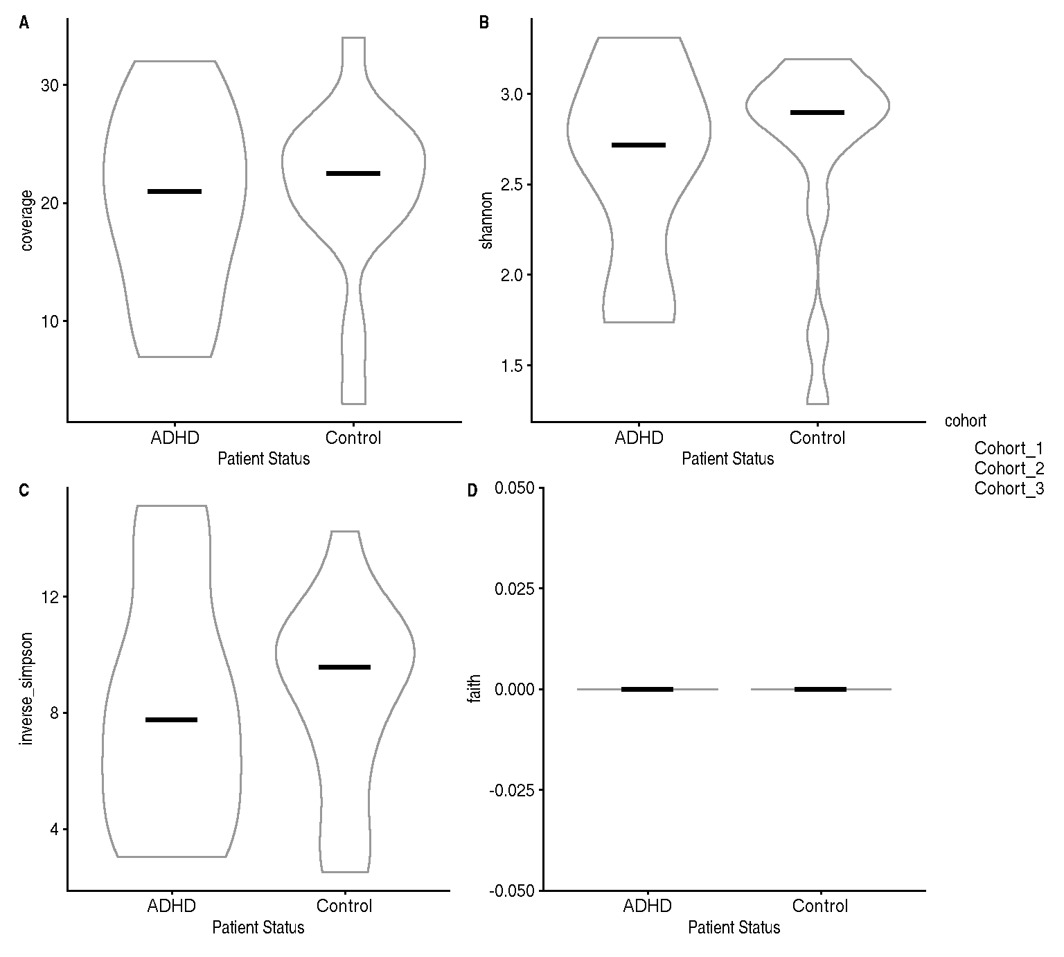
We calculate alpha diversity in terms of coverage, Shannon, inverse Simpson and Faith indices based on the counts assay. The first three indices differ from one another in how much weight they give to rare taxa: coverage considers all taxa equally important, whereas Shannon and - even more - Simpson give more importance to abundant taxa. Unlike all others, Faith index measures the phylogenetic diversity and thus requires a phylogenetic tree (stored as rowTree in the TreeSE).

# estimate the specified indices based on the counts assay
tse <- estimateDiversity(tse,
                         assay.type = "counts",
                         index = c("coverage", "shannon",
                                   "inverse_simpson", "faith"))

Visualisation

Next, we plot the four indices, with patient status on the x axis and alpha diversity on the y axis. We can also colour by cohort to check for batch effects.

# plot coverage vs patient_status
p_coverage <- plotColData(tse, "coverage", "patient_status",
                          colour_by = "cohort", show_median = TRUE) +
  labs(x = "Patient Status")

# plot shannon diversity vs patient_status
p_shannon <- plotColData(tse, "shannon", "patient_status",
                         colour_by = "cohort", show_median = TRUE) +
  labs(x = "Patient Status")

# plot inverse simpson index vs patient_status
p_simpson <- plotColData(tse, "inverse_simpson", "patient_status",
                         colour_by = "cohort", show_median = TRUE) +
  labs(x = "Patient Status")

# plot faith index vs patient_status
p_faith <- plotColData(tse, "faith", "patient_status",
                         colour_by = "cohort", show_median = TRUE) +
  labs(x = "Patient Status")

The three metrics for alpha diversity follow different scales, but they seem to agree when comparing the distributions of the two patient groups (see Figure 1).

# combine the plots with patchwork
p <- (p_coverage | p_shannon) / (p_simpson | p_faith) +
  plot_layout(guides = "collect") +
  plot_annotation(tag_levels = "A")
p

Figure 1: Box plots of (A) coverage (B) Shannon and (C) inverse Simpson indices grouped by patient status and coloured by cohort.