distance-based Redundance Analysis (dbRDA)

Overview

To get started, we import Tengeler2020 from the mia package and store it into a variable.

# load dataset and store it into tse
data("Tengeler2020", package = "mia")
tse <- Tengeler2020

First off, we transform the counts assay to relative abundances and store the new assay back in the TreeSE.

tse <- transformAssay(tse, method = "relabundance")

Ordination

RDA with Bray-Curtis index

tse <- runRDA(tse,
              formula = assay ~ patient_status + cohort,
              FUN = vegan::vegdist,
              method = "bray",
              assay.type = "relabundance")

p <- plotReducedDim(tse, "RDA",
                    colour_by = "patient_status",
                    shape_by = "cohort")

Figure 1: RDA plot with Bray-Curtis dissimilarity.

RDA with Aitchison distance

# perform clr transformation
tse <- transformAssay(tse,
                       assay.type = "relabundance",
                       method = "clr",
                       pseudocount = 1)

# run RDA
tse <- runRDA(tse,
              formula = assay ~ patient_status + cohort,
              FUN = vegan::vegdist,
              method = "euclidean",
              assay.type = "clr",
              name = "Aitchison")

# plot RDA
p <- plotReducedDim(tse, "Aitchison",
                    colour_by = "patient_status",
                    shape_by = "cohort")

Figure 2: RDA plot with Aitchison distance (CLR assay + Euclidian distance).

Significance testing

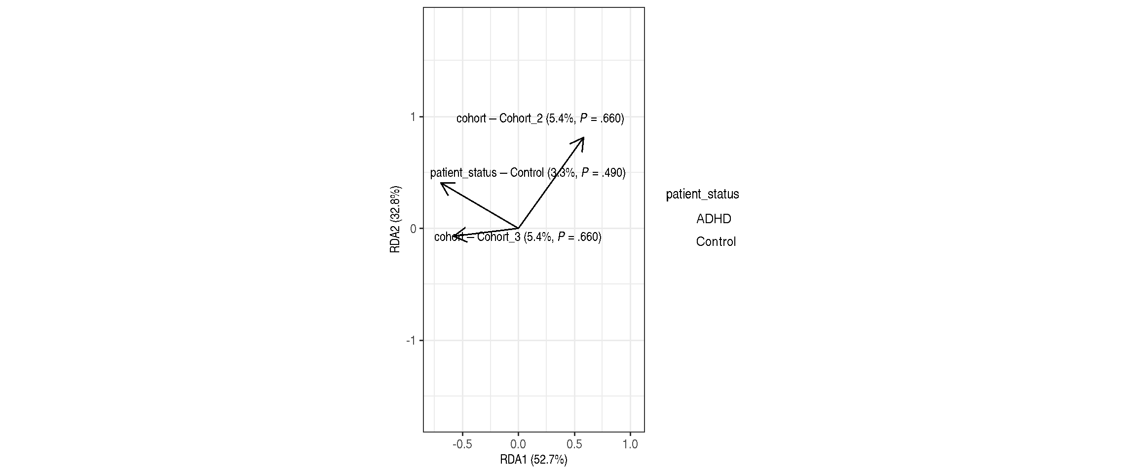
PERMANOVA analysis

rda <- attr(reducedDim(tse, "RDA"), "rda")

set.seed(123)
terms_permanova <- anova.cca(rda,
                             permutations = 99)

set.seed(123)
margin_permanova <- anova.cca(rda,
                              by = "margin",
                              permutations = 99)

Table 1: Results of PERMANOVA on patient_status and cohort groups.
	Df	SumOfSqs	F	Pr(>F)	Total variance	Explained variance
Model	3	0.1628626	0.7103337	0.70	1.920647	0.0847957
patient_status	1	0.0639173	0.8363361	0.49	1.920647	0.0332791
cohort	2	0.1042149	0.6818079	0.66	1.920647	0.0542603
Residual	23	1.7577847	NA	NA	1.920647	0.9152043

Test homogeneity assumption

homo1 <- anova(betadisper(vegdist(t(assay(tse, "relabundance"))), tse$patient_status))
homo2 <- anova(betadisper(vegdist(t(assay(tse, "relabundance"))), tse$cohort))

Table 2: Results of betadisper test on homogeneity.
	Df	Sum Sq	Mean Sq	F value	Pr(>F)
patient_status	1	0.0012087	0.0012087	0.0891227	0.7677628
cohort	2	0.0017934	0.0008967	0.0726010	0.9301753

RDA plot with weights