Chapter 5 Microbiome data exploration

Now we have loaded the data set into R. Next, let us walk through some basic operations for data exploration to confirm that the data has all the necessary components.

5.1 Data structure

Let us now investigate how taxonomic profiling data is organized in R.

Dimensionality tells us how many taxa and samples the data contains. As we can see, there are 12613 taxa and 40 samples.

# mae[[1]]: indexing/retrieving the taxonomic data experiment
dim(mae[[1]])

## [1] 12613    40

The rowData slot contains a taxonomic table. This includes taxonomic information for each of the 12613 entries. With the head() command, we can print just the beginning of the table.

The rowData seems to contain information from 7 different taxonomy classes.

knitr::kable(head(rowData(mae[[1]]))) %>% 
  kableExtra::kable_styling("striped", 
                            latex_options="scale_down") %>% 
  kableExtra::scroll_box(width = "100%")

	Phylum	Class	Order	Family	Genus	Species	OTU
GAYR01026362.62.2014	Proteobacteria	Alphaproteobacteria	Rickettsiales	Mitochondria	Solanum melongena (eggplant)	Solanum melongena (eggplant)	GAYR01026362.62.2014
CVJT01000011.50.2173	Firmicutes	Bacilli	Bacillales	Staphylococcaceae	Staphylococcus	Staphylococcus aureus	CVJT01000011.50.2173
KF625183.1.1786	Proteobacteria	Gammaproteobacteria	Enterobacteriales	Enterobacteriaceae	Klebsiella	Klebsiella oxytoca	KF625183.1.1786
AYSG01000002.292.2076	Firmicutes	Bacilli	Lactobacillales	Streptococcaceae	Streptococcus	Streptococcus thermophilus TH1435	AYSG01000002.292.2076
CCPS01000022.154.1916	Proteobacteria	Gammaproteobacteria	Enterobacteriales	Enterobacteriaceae	Escherichia-Shigella	Escherichia coli	CCPS01000022.154.1916
KJ923794.1.1762	Firmicutes	Bacilli	Bacillales	Staphylococcaceae	Staphylococcus	Staphylococcus aureus	KJ923794.1.1762

The colData slot contains sample metadata. It contains information for all 40 samples. However, here only the 6 first samples are shown as we use the head() command. There are 6 columns, that contain information, e.g., about patients’ status, and cohort.

# For simplicity, classify all high-fat diets as high-fat, and all the low-fat 
# diets as low-fat diets
colData(mae)$Diet <- ifelse(colData(mae)$Diet == "High-fat" | 
                              colData(mae)$Diet == "High-fat + XOS", 
                            "High-fat", "Low-fat")

knitr::kable(head(colData(mae))) %>% 
  kableExtra::kable_styling("striped", 
                            latex_options="scale_down") %>% 
  kableExtra::scroll_box(width = "100%")

	Sample	Rat	Site	Diet	Fat
C1	C1	1	Cecum	High-fat	High
C2	C2	2	Cecum	High-fat	High
C3	C3	3	Cecum	High-fat	High
C4	C4	4	Cecum	High-fat	High
C5	C5	5	Cecum	High-fat	High
C6	C6	6	Cecum	High-fat	High

From here, we can draw summaries of the sample (column) data, for instance to see what is the diet distribution.

The command colData(mae)$Diet fetches the data from the column, and table() creates a table that shows how many times each class is present, and sort() sorts the table to ascending order.

There are 20 samples from mice having High-fat, and 20 Low-fat.

sort(table(colData(mae)$Diet))

## 
## High-fat  Low-fat 
##       20       20

5.1.1 Transformations

Microbial abundances are typically ‘compositional’ (relative) in the current microbiome profiling data sets. This is due to technical aspects of the data generation process (see e.g. Gloor et al., 2017).

The next example calculates relative abundances as these are usually easier to interpret than plain counts. For some statistical models we need to transform the data into other formats as explained in above link (and as we will see later).

# Calculates relative abundances, and stores the table to assays
mae[[1]] <- transformCounts(mae[[1]], method = "relabundance")

A variety of standard transformations for microbiome data are available through mia R package.

5.1.2 Aggregation

Microbial species can be called at multiple taxonomic resolutions. We can easily agglomerate the data based on taxonomic ranks. Here, we agglomerate the data at Phylum level.

se_phylum <- agglomerateByRank(mae[[1]], rank = "Phylum")

# Show dimensionality
dim(se_phylum)

## [1] 13 40

Now there are 13 taxa and 40 samples, meaning that there are 13 different Phylum level taxonomic groups. Looking at the rowData after agglomeration shows all Firmicutes are combined together, and all lower rank information is lost.

From the assay we can see that all abundances of taxa that belong to Firmicutes are summed up.

knitr::kable(head(rowData(se_phylum))) %>% 
  kableExtra::kable_styling("striped", 
                            latex_options="scale_down") %>% 
  kableExtra::scroll_box(width = "100%")

	Phylum	Class	Order	Family	Genus	Species	OTU
Proteobacteria	Proteobacteria	NA	NA	NA	NA	NA	GAYR01026362.62.2014
Firmicutes	Firmicutes	NA	NA	NA	NA	NA	CVJT01000011.50.2173
Cyanobacteria	Cyanobacteria	NA	NA	NA	NA	NA	GEMN01027092.33.1623
Tenericutes	Tenericutes	NA	NA	NA	NA	NA	AM277369.1.1548
Deferribacteres	Deferribacteres	NA	NA	NA	NA	NA	AYGZ01000001.327.1863
Actinobacteria	Actinobacteria	NA	NA	NA	NA	NA	JGZF01000005.1.1534

If you are sharp, you have by now noticed that all the aggregated values in the above example are NA’s (missing data). This is because the agglomeration is missing abundances for certain taxa, and in that case the sum is not defined by default (na.rm = FALSE). We can ignore the missing values in summing up the data by setting na.rm = TRUE; then the taxa that do not have information in specified level will be removed. Those taxa that do not have information in specified level are agglomerated at lowest possible level that is left after agglomeration.

temp <- rowData(agglomerateByRank(mae[[1]], rank = "Genus"))

# Prints those taxa that do not have information at the Genus level (NA)
knitr::kable(head(temp[which(is.na(temp$Genus)),])) %>% 
  kableExtra::kable_styling("striped", 
                            latex_options="scale_down") %>% 
  kableExtra::scroll_box(width = "100%")

	Phylum	Class	Order	Family	Genus	Species	OTU
Family:uncultured	Proteobacteria	Alphaproteobacteria	Rhodospirillales	uncultured	NA	NA	JRJTB:01000:00983
Family:Ruminococcaceae	Firmicutes	Clostridia	Clostridiales	Ruminococcaceae	NA	NA	JRJTB:00751:00256
Order:Clostridiales	Firmicutes	Clostridia	Clostridiales	NA	NA	NA	JRJTB:03059:01977
Family:Lachnospiraceae	Firmicutes	Clostridia	Clostridiales	Lachnospiraceae	NA	NA	JRJTB:00738:02832
Family:Peptostreptococcaceae	Firmicutes	Clostridia	Clostridiales	Peptostreptococcaceae	NA	NA	JRJTB:01731:00274
Family:Pasteurellaceae	Proteobacteria	Gammaproteobacteria	Pasteurellales	Pasteurellaceae	NA	NA	JRJTB:01960:01703

Here agglomeration is done similarly, but na.rm = TRUE

temp2 <- rowData(agglomerateByRank(mae[[1]], rank = "Genus", na.rm = TRUE))

print(paste0("Agglomeration with na.rm = FALSE: ", dim(temp)[1], " taxa."))

## [1] "Agglomeration with na.rm = FALSE: 277 taxa."

print(paste0("Agglomeration with na.rm = TRUE: ", dim(temp2)[1], " taxa."))

## [1] "Agglomeration with na.rm = TRUE: 262 taxa."

The mia package contains further examples on various data agglomeration and splitting options.

5.2 Visualization

The miaViz package facilitates data visualization. Let us plot the Phylum level abundances.

# Here we specify "relabundance" to be abundance table that we use for plotting.
# Note that we can use agglomerated or non-agglomerated mae[[1]] as an input, because
# the function agglomeration is built-in option. 

# Legend does not fit into picture, so its height is reduced.
plot_abundance <- plotAbundance(mae[[1]], abund_values="relabundance", rank = "Phylum") +
  theme(legend.key.height = unit(0.5, "cm")) +
  scale_y_continuous(label = scales::percent)

plot_abundance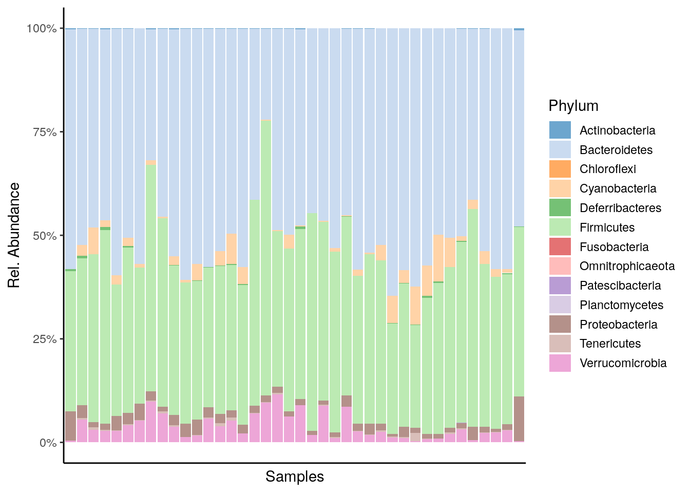

Density plot shows the overall abundance distribution for a given taxonomic group. Let us check the relative abundance of Firmicutes across the sample collection. The density plot is a smoothened version of a standard histogram.

The plot shows peak abundances around 30 %.

# Subset data by taking only Firmicutes
se_firmicutes <- se_phylum["Firmicutes"]

# Gets the abundance table
abundance_firmicutes <- assay(se_firmicutes, "relabundance")

# Creates a data frame object, where first column includes abundances
firmicutes_abund_df <- as.data.frame(t(abundance_firmicutes))
# Rename the first and only column
colnames(firmicutes_abund_df) <- "abund"

# Creates a plot. Parameters inside feom_density are optional. With 
# geom_density(bw=1000), it is possible to adjust bandwidth.
firmicutes_abund_plot <- ggplot(firmicutes_abund_df, aes(x = abund)) + 
  geom_density(color="darkred", fill="lightblue") + 
  labs(x = "Relative abundance", title = "Firmicutes") +
  theme_classic() + # Changes the background
  scale_x_continuous(label = scales::percent)

firmicutes_abund_plot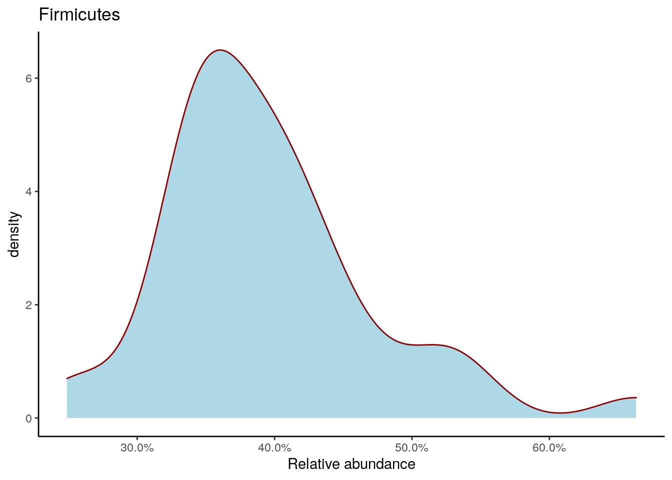

For more visualization options and examples, see the miaViz vignette.