Apply a function by feature or sample group

applyByModule provides a convenient method to apply the same operation on multiple, possibly overlapping groups of features or samples, representing for example functional microbial modules or sample categories, respectively.

applyByModule(x, ...)

# S4 method for class 'SummarizedExperiment'
applyByModule(
  x,
  .by,
  .group,
  FUN,
  min.group.size = NULL,
  meta.name = "mod_res",
  ...
)

Arguments

x

A SummarizedExperiment object.

...

Additional arguments passed to FUN.

.by

Character scalar. Whether .group information pertains the "rows" or "cols" of x.

.group

Character vector. Names of the groups or modules by which FUN is applied.

FUN

Function scalar. A function which takes x as the first argument and ... as additional arguments. To update x in place, use get and not add functions, as the latter will populate the altExp slot.

min.group.size

Numeric scalar. The minimum number of features or samples in a group for FUN to be applied. (Default: NULL)

meta.name

Character scalar. The name of the metadata slot where results are stored. (Default: "mod.res")

Value

x updated with results stored in the appropriate slot depending on the given FUN.

Details

It is recommended to use get* functions to store results in the appropriate slot of x, whereas using the add* functions applied to features will save the results as separate experiments in the altExp slot. In summary, function results are stored as follows:

• colData: getAlpha, getDominance, getPrevalence, getCluster

• reducedDims: getMDS, getNMDS, getCCA, getRDA, getLDA, getNMF, getDPCoA, calculatePCA

• altExps: transformAssay and add* functions

• metadata: all else (miaViz ggplot2 objects, statistical summaries, etc.)

Examples

library(bluster)
library(miaViz)
#> Loading required package: ggraph
#> 
#> Attaching package: ‘miaViz’
#> The following object is masked from ‘package:scater’:
#> 
#>     plotHeatmap
#> The following object is masked from ‘package:mia’:
#> 
#>     plotNMDS
library(patchwork)

# Import dataset
data("Tengeler2020", package = "mia")
tse <- Tengeler2020

# Compute alpha diversity indices for each Order
tse <- applyByModule(
    tse,
    .by = "rows",
    .group = "Order",
    FUN = getAlpha,
    index = c("shannon", "faith"),
    min.group.size = 2
)

# View colData names for alpha diversity results
names(colData(tse))
#>  [1] "patient_status"             "cohort"                    
#>  [3] "patient_status_vs_cohort"   "sample_name"               
#>  [5] "shannon_Bacteroidales"      "faith_Bacteroidales"       
#>  [7] "shannon_Clostridiales"      "faith_Clostridiales"       
#>  [9] "shannon_Enterobacteriales"  "faith_Enterobacteriales"   
#> [11] "shannon_Erysipelotrichales" "faith_Erysipelotrichales"  
#> [13] "shannon_Verrucomicrobiales" "faith_Verrucomicrobiales"  

# Compute beta diversity measures for each Order
tse <- applyByModule(
    tse,
    .by = "rows",
    .group = "Order",
    FUN = getMDS,
    method = "unifrac",
    min.group.size = 2
)

# View reducedDim names for beta diversity results
reducedDimNames(tse)
#> [1] "Bacteroidales"      "Clostridiales"      "Enterobacteriales" 
#> [4] "Erysipelotrichales" "Verrucomicrobiales"

# Transform assay for each Order, storing results as altExps
tse <- applyByModule(
    tse,
    .by = "rows",
    .group = "Order",
    FUN = transformAssay,
    method = "clr",
    pseudocount = TRUE
)

# View altExp names for newly transformed assays
altExpNames(tse)
#> [1] "Bacteroidales"       "Clostridiales"       "Enterobacteriales"  
#> [4] "Erysipelotrichales"  "Gastranaerophilales" "Oceanospirillales"  
#> [7] "Verrucomicrobiales" 

# Create two example microbial modules
rowData(tse)$Mod1 <- rowData(tse)$Family == "Ruminococcaceae"
rowData(tse)$Mod2 <- rowData(tse)$Order == "Clostridiales"

# Find sample-wise most dominant genus for each module
tse <- applyByModule(
    tse,
    .by = "rows",
    .group = c("Mod1", "Mod2"),
    FUN = getDominant,
    group = "Genus"
)

# View colData names for dominance results
names(colData(tse))
#>  [1] "patient_status"             "cohort"                    
#>  [3] "patient_status_vs_cohort"   "sample_name"               
#>  [5] "shannon_Bacteroidales"      "faith_Bacteroidales"       
#>  [7] "shannon_Clostridiales"      "faith_Clostridiales"       
#>  [9] "shannon_Enterobacteriales"  "faith_Enterobacteriales"   
#> [11] "shannon_Erysipelotrichales" "faith_Erysipelotrichales"  
#> [13] "shannon_Verrucomicrobiales" "faith_Verrucomicrobiales"  
#> [15] "dominant_Mod1"              "dominant_Mod2"             

# Cluster samples by features for each module
tse <- applyByModule(
    tse,
    .by = "rows",
    .group = c("Mod1", "Mod2"),
    FUN = getCluster,
    assay.type = "counts",
    by = "cols",
    BLUSPARAM = KmeansParam(centers = 3)
)

# View colData names for clustering results
names(colData(tse))
#>  [1] "patient_status"             "cohort"                    
#>  [3] "patient_status_vs_cohort"   "sample_name"               
#>  [5] "shannon_Bacteroidales"      "faith_Bacteroidales"       
#>  [7] "shannon_Clostridiales"      "faith_Clostridiales"       
#>  [9] "shannon_Enterobacteriales"  "faith_Enterobacteriales"   
#> [11] "shannon_Erysipelotrichales" "faith_Erysipelotrichales"  
#> [13] "shannon_Verrucomicrobiales" "faith_Verrucomicrobiales"  
#> [15] "dominant_Mod1"              "dominant_Mod2"             
#> [17] "cluster_Mod1"               "cluster_Mod2"              

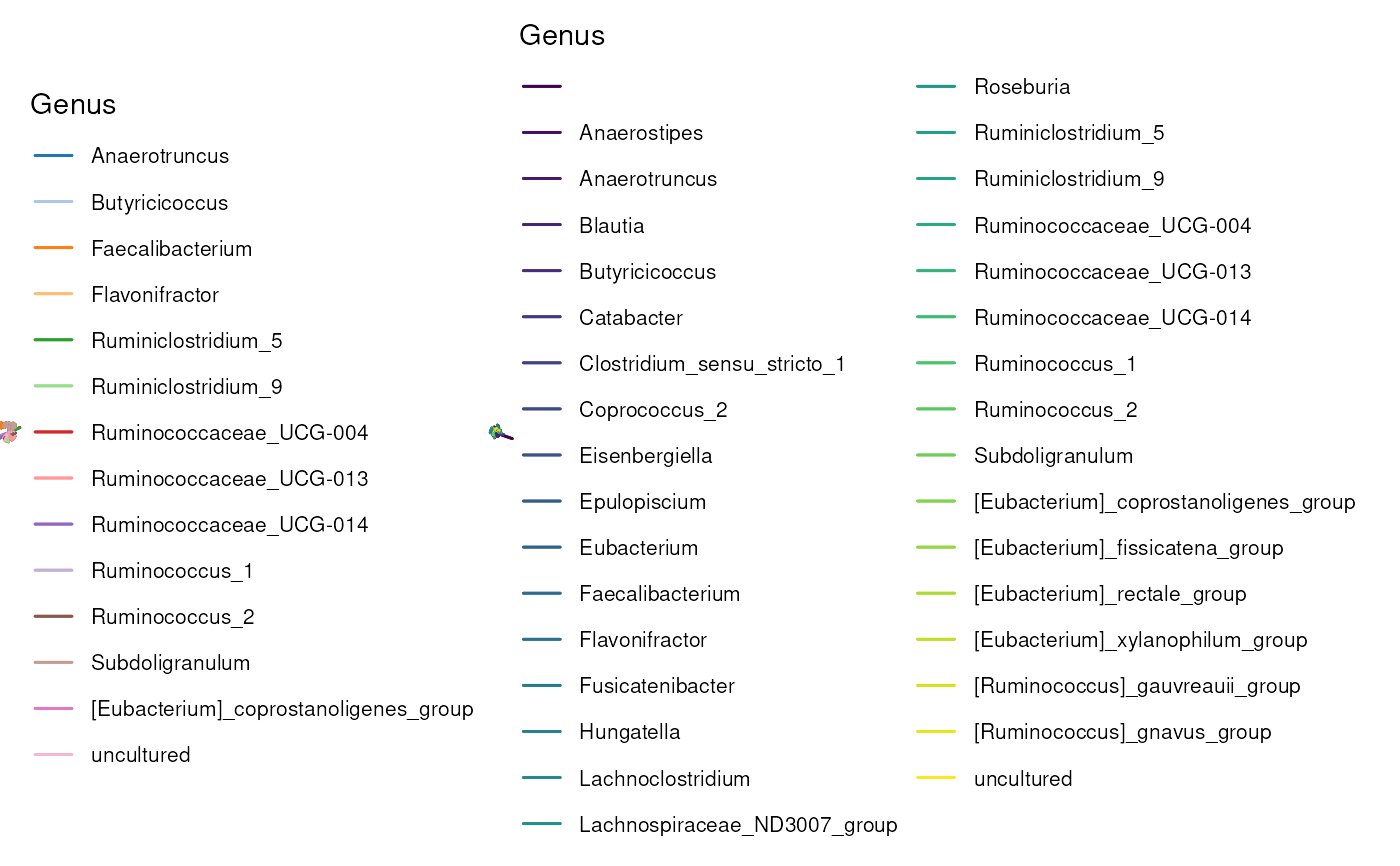
# Plot tree for each module, specifying metadata name
tse <- applyByModule(
    tse,
    .by = "rows",
    .group = c("Mod1", "Mod2"),
    FUN = plotRowTree,
    edge.colour.by = "Genus",
    meta.name = "tree_plots"
)

# Visualize module-wise abundance plots
metadata(tse)$tree_plots |>
    wrap_plots()