Data Manipulation
Why data manipulation?
Raw data might be uninformative or incompatible with a method. We want to be able to modify, polish, subset, agglomerate and transform it.

Why so complex?
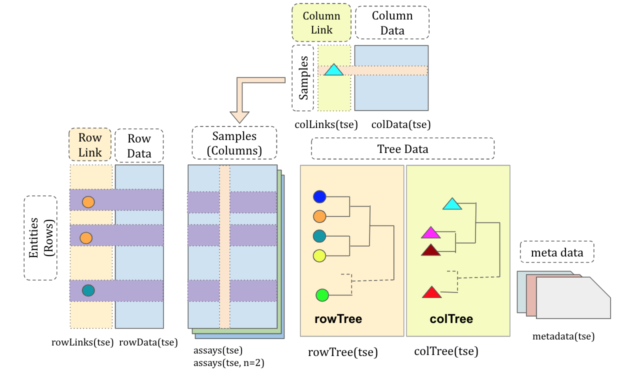
TreeSE containers organise information to improve flexibility and accessibility, which comes with a bit of complexity. Focus on assays, colData and rowData.

Example 1.1: Data Import
We work with microbiome data inside TreeSummarizedExperiment (TreeSE) containers and mia is our toolkit.
The components of a TreeSE can all be seen at a glance.
class: TreeSummarizedExperiment
dim: 151 27
metadata(0):
assays(1): counts
rownames(151): Bacteroides Bacteroides_1 ... Parabacteroides_8
  Unidentified_Lachnospiraceae_14
rowData names(6): Kingdom Phylum ... Family Genus
colnames(27): A110 A12 ... A35 A38
colData names(4): patient_status cohort patient_status_vs_cohort
  sample_name
reducedDimNames(0):
mainExpName: NULL
altExpNames(0):
rowLinks: a LinkDataFrame (151 rows)
rowTree: 1 phylo tree(s) (151 leaves)
colLinks: NULL
colTree: NULL
Example 1.2: Column data
Columns represent the samples of an experiment.
All information about the samples is stored in colData.
DataFrame with 3 rows and 4 columns
     patient_status      cohort patient_status_vs_cohort sample_name
        <character> <character>              <character> <character>
A110           ADHD    Cohort_1            ADHD_Cohort_1        A110
A12            ADHD    Cohort_1            ADHD_Cohort_1         A12
A15            ADHD    Cohort_1            ADHD_Cohort_1         A15
Individual variables about the samples can be accessed directly.
Example 1.3: Row data
Rows represent the features of an experiment.
All information about the samples is stored in rowData.
DataFrame with 3 rows and 6 columns
                    Kingdom        Phylum       Class         Order
                <character>   <character> <character>   <character>
Bacteroides        Bacteria Bacteroidetes Bacteroidia Bacteroidales
Bacteroides_1      Bacteria Bacteroidetes Bacteroidia Bacteroidales
Parabacteroides    Bacteria Bacteroidetes Bacteroidia Bacteroidales
                            Family           Genus
                       <character>     <character>
Bacteroides         Bacteroidaceae     Bacteroides
Bacteroides_1       Bacteroidaceae     Bacteroides
Parabacteroides Porphyromonadaceae Parabacteroides
Individual variables about the samples can be accessed from rowData.
Example 1.4: Assays
The assays of an experiment (counts, relative abundance, etc.) can be found in assays.
assayNames return only their names.
An individual assay can be retrieved with assay.
Exercise 1
- preliminary exploration: exercise 3.3
- assay retrieval: exercise 3.4
Extra:
- constructing a TreeSE object: exercise 3.1
Raw data can be retrieved here.
Example 2.1: Subsetting
We can subset features or samples of a TreeSE, but first we need to pick a variable.
To subset samples, we filter columns with a conditional.
[1] 151 13We now want to subset by our favourite Phylum.
[1] "Bacteroidetes"   "Verrucomicrobia" "Proteobacteria"  "Firmicutes"
[5] "Cyanobacteria"
To subset features, we filter rows with a conditional.
Example 2.2: Agglomeration
Agglomeration condenses the assays to higher taxonomic ranks. Related taxa are combined together. We can agglomerate by different ranks.
We agglomerate by Phylum and store the new experiment in the altExp slot.
# Agglomerate by Phylum and store into altExp slot
altExp(tse, "phylum") <- agglomerateByRank(tse, rank = "Phylum")
altExp(tse, "phylum")
class: TreeSummarizedExperiment
dim: 5 27
metadata(1): agglomerated_by_rank
assays(1): counts
rownames(5): Bacteroidetes Cyanobacteria Firmicutes Proteobacteria
Verrucomicrobia
rowData names(6): Kingdom Phylum ... Family Genus
colnames(27): A110 A12 ... A35 A38
colData names(4): patient_status cohort patient_status_vs_cohort
sample_name
reducedDimNames(0):
mainExpName: NULL
altExpNames(0):
rowLinks: a LinkDataFrame (5 rows)
rowTree: 1 phylo tree(s) (151 leaves)
colLinks: NULL
colTree: NULLExample 2.3: Transformation
Data can be transformed for different reasons. For example, to make samples comparable we can use relative abundance.
# Transform counts to relative abundance
tse <- transformAssay(tse,
                      assay.type = "counts",
                      method = "relabundance")

# View sample-wise sums
head(colSums(assay(tse, "relabundance")), 3)
A110 A12 A15
1 1 1 Or to standardise features to the normal distribution we can use z-scores: \(Z = \frac{x - \mu}{\sigma}\).
Exercise 2
- subsetting: exercise 4.1
- agglomeration: exercise 5.1
- transformation: exercise 4.6
Extra:
- prevalence subsetting: exercise 4.3
- alternative experiments: exercise 5.2
Resources
- mia function reference
- OMA Section - Data Containers
- OMA Section - Subsetting
- OMA Section - Agglomeration
- OMA Section - Transformation