2 Microbiome Data

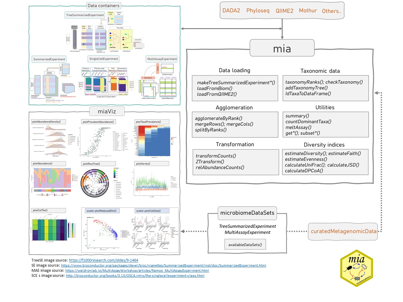
2.1 Data science framework

The building blocks of the framework are data container (SummarizedExperiment and its derivatives), packages from various developers using the TreeSE container, open demonstration data sets, in a separate chapter Section 2.3, and online tutorials including this online book as well as the various package vignettes and other materials.

2.2 Data containers

SummarizedExperiment (SE) (Morgan et al. 2020) is a generic and highly optimized container for complex data structures. It has become a common choice for analysing various types of biomedical profiling data, such as RNAseq, ChIp-Seq, microarrays, flow cytometry, proteomics, and single-cell sequencing.

Morgan, Martin, Valerie Obenchain, Jim Hester, and Hervé Pagès. 2020. SummarizedExperiment: SummarizedExperiment Container. https://bioconductor.org/packages/SummarizedExperiment.

Huang, Ruizhu. 2020. TreeSummarizedExperiment: A S4 Class for Data with Tree Structures.

[TreeSummarizedExperiment] (TreeSE) (Huang 2020) was developed as an extension to incorporate hierarchical information (such as phylogenetic trees and sample hierarchies) and reference sequences.

[MultiAssayExperiment] (MAE) (Ramos et al. 2017) provides an organized way to bind several different data containers together in a single object. For example, we can bind microbiome data (in TreeSE container) with metabolomic profiling data (in SE) container, with (partially) shared sample metadata. This is convenient and robust for instance in subsetting and other data manipulation tasks. Microbiome data can be part of multiomics experiments and analysis strategies. We highlight how the methods used througout in this book relate to this data framework by using the TreeSummarizedExperiment, MultiAssayExperiment, and classes beyond.

This section provides an introductions to these data containers. In microbiome data science, these containers link taxonomic abundance tables with rich side information on the features and samples. Taxonomic abundance data can be obtained by 16S rRNA amplicon or metagenomic sequencing, phylogenetic microarrays, or by other means. Many microbiome experiments include multiple versions and types of data generated independently or derived from each other through transformation or agglomeration. We start by providing recommendations on how to represent different varieties of multi-table data within the TreeSummarizedExperiment class.

The options and recommendations are summarized in Table 2.1.

2.2.1 Assay data

The original count-based taxonomic abundance tables may have different transformations, such as logarithmic, Centered Log-Ratio (CLR), or relative abundance. These are typically stored in assays.

Let us load example data and rename it as tse.

library(mia)
data("GlobalPatterns", package = "mia")
tse <- GlobalPatterns

The assays slot contains the experimental data as multiple count matrices. The result of assays is a list of matrices.

assays(tse)
##  List of length 1
##  names(1): counts

Individual assays can be accessed via assay

assay(tse, "counts")[1:5,1:7]
##         CL3 CC1 SV1 M31Fcsw M11Fcsw M31Plmr M11Plmr
##  549322   0   0   0       0       0       0       0
##  522457   0   0   0       0       0       0       0
##  951      0   0   0       0       0       0       1
##  244423   0   0   0       0       0       0       0
##  586076   0   0   0       0       0       0       0

To illustrate the use of multiple assays, the relative abundance data can be calculated and stored along the original count data using transformAssay.

tse <- transformAssay(tse, assay.type = "counts", method = "relabundance")
assays(tse)
##  List of length 2
##  names(2): counts relabundance

Now there are two assays available in the tse object, counts and relabundance.

assay(tse, "relabundance")[1:5,1:7]
##         CL3 CC1 SV1 M31Fcsw M11Fcsw M31Plmr   M11Plmr
##  549322   0   0   0       0       0       0 0.000e+00
##  522457   0   0   0       0       0       0 0.000e+00
##  951      0   0   0       0       0       0 2.305e-06
##  244423   0   0   0       0       0       0 0.000e+00
##  586076   0   0   0       0       0       0 0.000e+00

Here the dimension of the count data remains unchanged in transformation. This is in fact, a requirement for the assays.

2.2.2 colData

colData contains data on the samples.

colData(tse)
##  DataFrame with 26 rows and 7 columns
##          X.SampleID   Primer Final_Barcode Barcode_truncated_plus_T
##            <factor> <factor>      <factor>                 <factor>
##  CL3        CL3      ILBC_01        AACGCA                   TGCGTT
##  CC1        CC1      ILBC_02        AACTCG                   CGAGTT
##  SV1        SV1      ILBC_03        AACTGT                   ACAGTT
##  M31Fcsw    M31Fcsw  ILBC_04        AAGAGA                   TCTCTT
##  M11Fcsw    M11Fcsw  ILBC_05        AAGCTG                   CAGCTT
##  ...            ...      ...           ...                      ...
##  TS28         TS28   ILBC_25        ACCAGA                   TCTGGT
##  TS29         TS29   ILBC_26        ACCAGC                   GCTGGT
##  Even1        Even1  ILBC_27        ACCGCA                   TGCGGT
##  Even2        Even2  ILBC_28        ACCTCG                   CGAGGT
##  Even3        Even3  ILBC_29        ACCTGT                   ACAGGT
##          Barcode_full_length SampleType
##                     <factor>   <factor>
##  CL3             CTAGCGTGCGT      Soil 
##  CC1             CATCGACGAGT      Soil 
##  SV1             GTACGCACAGT      Soil 
##  M31Fcsw         TCGACATCTCT      Feces
##  M11Fcsw         CGACTGCAGCT      Feces
##  ...                     ...        ...
##  TS28            GCATCGTCTGG      Feces
##  TS29            CTAGTCGCTGG      Feces
##  Even1           TGACTCTGCGG      Mock 
##  Even2           TCTGATCGAGG      Mock 
##  Even3           AGAGAGACAGG      Mock 
##                                         Description
##                                            <factor>
##  CL3     Calhoun South Carolina Pine soil, pH 4.9  
##  CC1     Cedar Creek Minnesota, grassland, pH 6.1  
##  SV1     Sevilleta new Mexico, desert scrub, pH 8.3
##  M31Fcsw M3, Day 1, fecal swab, whole body study   
##  M11Fcsw M1, Day 1, fecal swab, whole body study   
##  ...                                            ...
##  TS28                                       Twin #1
##  TS29                                       Twin #2
##  Even1                                      Even1  
##  Even2                                      Even2  
##  Even3                                      Even3

2.2.3 rowData

rowData contains data on the features of the analyzed samples. Of particular interest to the microbiome field, this is used to store taxonomic information.

rowData(tse)
##  DataFrame with 19216 rows and 7 columns
##             Kingdom        Phylum        Class        Order        Family
##         <character>   <character>  <character>  <character>   <character>
##  549322     Archaea Crenarchaeota Thermoprotei           NA            NA
##  522457     Archaea Crenarchaeota Thermoprotei           NA            NA
##  951        Archaea Crenarchaeota Thermoprotei Sulfolobales Sulfolobaceae
##  244423     Archaea Crenarchaeota        Sd-NA           NA            NA
##  586076     Archaea Crenarchaeota        Sd-NA           NA            NA
##  ...            ...           ...          ...          ...           ...
##  278222    Bacteria           SR1           NA           NA            NA
##  463590    Bacteria           SR1           NA           NA            NA
##  535321    Bacteria           SR1           NA           NA            NA
##  200359    Bacteria           SR1           NA           NA            NA
##  271582    Bacteria           SR1           NA           NA            NA
##               Genus                Species
##         <character>            <character>
##  549322          NA                     NA
##  522457          NA                     NA
##  951     Sulfolobus Sulfolobusacidocalda..
##  244423          NA                     NA
##  586076          NA                     NA
##  ...            ...                    ...
##  278222          NA                     NA
##  463590          NA                     NA
##  535321          NA                     NA
##  200359          NA                     NA
##  271582          NA                     NA

2.2.4 rowTree

Phylogenetic trees also play an important role in the microbiome field. The TreeSummarizedExperiment class can keep track of features and node relations via two functions, rowTree and rowLinks.

A tree can be accessed via rowTree as phylo object.

rowTree(tse)
##  
##  Phylogenetic tree with 19216 tips and 19215 internal nodes.
##  
##  Tip labels:
##    549322, 522457, 951, 244423, 586076, 246140, ...
##  Node labels:
##    , 0.858.4, 1.000.154, 0.764.3, 0.995.2, 1.000.2, ...
##  
##  Rooted; includes branch lengths.

The links to the individual features are available through rowLinks.

rowLinks(tse)
##  LinkDataFrame with 19216 rows and 5 columns
##            nodeLab   nodeNum nodeLab_alias    isLeaf   whichTree
##        <character> <integer>   <character> <logical> <character>
##  1          549322         1       alias_1      TRUE       phylo
##  2          522457         2       alias_2      TRUE       phylo
##  3             951         3       alias_3      TRUE       phylo
##  4          244423         4       alias_4      TRUE       phylo
##  5          586076         5       alias_5      TRUE       phylo
##  ...           ...       ...           ...       ...         ...
##  19212      278222     19212   alias_19212      TRUE       phylo
##  19213      463590     19213   alias_19213      TRUE       phylo
##  19214      535321     19214   alias_19214      TRUE       phylo
##  19215      200359     19215   alias_19215      TRUE       phylo
##  19216      271582     19216   alias_19216      TRUE       phylo

Please note that there can be a 1:1 relationship between tree nodes and features, but this is not a must-have. This means there can be features, which are not linked to nodes, and nodes, which are not linked to features. To change the links in an existing object, the changeTree function is available.

2.2.5 Alternative experiments

Alternative experiments complement assays. They can contain complementary data, which is no longer tied to the same dimensions as the assay data. However, the number of samples (columns) must be the same.

This can come into play, for instance, when one has taxonomic abundance profiles quantified with different measurement technologies, such as phylogenetic microarrays, amplicon sequencing, or metagenomic sequencing. Another common use case is including abundance tables for different taxonomic ranks. Such alternative experiments concerning the same set of samples can be stored as

Separate assays assuming that the taxonomic information can be mapped between features directly 1:1; or
Data in the altExp slot of the TreeSummarizedExperiment, if the feature dimensions differ. Each element of the altExp slot is a SummarizedExperiment or an object from a derived class with independent feature data.

The following shows how to store taxonomic abundance tables agglomerated at different taxonomic levels. However, the data could as well originate from entirely different measurement sources as long as the samples match.

Let us first agglomerate the data to Phylum level. This yields a new TreeSE data object.

tse_phylum <- mergeFeaturesByRank(tse, "Phylum", na.rm=TRUE)
# Both have the same number of columns (samples)
dim(tse)
##  [1] 19216    26
dim(tse_phylum)
##  [1] 66 26

Then we can add the new phylum-level data object as an alternative experiment in the original data.

# Add the new data object to the original data object as an alternative experiment with the name "Phylum"
altExp(tse, "Phylum") <- tse_phylum

# Check the alternative experiment names available in the data
altExpNames(tse)
##  [1] "Phylum"

We can now subset the data, for instance, and this acts on both altExp and assay data.

tse[,1:10]
##  class: TreeSummarizedExperiment 
##  dim: 19216 10 
##  metadata(0):
##  assays(2): counts relabundance
##  rownames(19216): 549322 522457 ... 200359 271582
##  rowData names(7): Kingdom Phylum ... Genus Species
##  colnames(10): CL3 CC1 ... M31Tong M11Tong
##  colData names(7): X.SampleID Primer ... SampleType Description
##  reducedDimNames(0):
##  mainExpName: NULL
##  altExpNames(1): Phylum
##  rowLinks: a LinkDataFrame (19216 rows)
##  rowTree: 1 phylo tree(s) (19216 leaves)
##  colLinks: NULL
##  colTree: NULL
dim(altExp(tse[,1:10],"Phylum"))
##  [1] 66 10

For more details on altExp, you can check the introduction to the SingleCellExperiment package (Lun and Risso 2020).

Lun, Aaron, and Davide Risso. 2020. SingleCellExperiment: S4 Classes for Single Cell Data.

2.2.6 MultiAssayExperiments

Multiple experiments relate to complementary measurement types, such as transcriptomic or metabolomic profiling of the microbiome or the host. Multiple experiments can be represented using the same options as alternative experiments, or by using the MultiAssayExperiment class (Ramos et al. 2017). Depending on how the datasets relate to each other the data can be stored as:

Ramos, Marcel, Lucas Schiffer, Angela Re, Rimsha Azhar, Azfar Basunia, Carmen Rodriguez Cabrera, Tiffany Chan, et al. 2017. “Software for the Integration of Multiomics Experiments in Bioconductor.” Cancer Research. https://doi.org/10.1158/0008-5472.CAN-17-0344.

Separate altExp if the samples can be matched directly 1:1; or
As MultiAssayExperiment objects, in which the connections between samples are defined through a sampleMap. Each element on the experimentsList of an MultiAssayExperiment is matrix or matrix-like objects, including SummarizedExperiment objects, and the number of samples can differ between the elements.

For information have a look at the intro vignette of the MultiAssayExperiment package.

Table 2.1: **Recommended options for storing multiple data tables in microbiome studies** The *assays* are best suited for data transformations (one-to-one match between samples and columns across the assays). The *alternative experiments* are particularly suitable for alternative versions of the data that are of same type but may have a different number of features (e.g. taxonomic groups); this is for instance the case with taxonomic abundance tables agglomerated at different levels (e.g. genus vs. phyla) or alternative profiling technologies (e.g. amplicon sequencing vs. shallow shotgun metagenomics). For alternative experiments one-to-one match between samples (cols) is libraryd but the alternative experiment tables can have different numbers of features (rows). Finally, elements of the *MultiAssayExperiment* provide the most flexible way to incorporate multi-omic data tables with flexible numbers of samples and features. We recommend these conventions as the basis for methods development and application in microbiome studies.
Option	Rows (features)	Cols (samples)	Recommended
assays	match	match	Data transformations
altExp	free	match	Alternative experiments
MultiAssay	free	free (mapping)	Multi-omic experiments

2.3 Demonstration data

Open demonstration data for testing and benchmarking purposes is available from multiple locations. This chapter introduces some options. The other chapters of this book provide ample examples about the use of the data.

2.3.1 Package data

The mia R package contains example datasets that are direct conversions from the alternative phyloseq container to the TreeSummarizedExperiment container.

List the available datasets in the mia package:

library(mia)
data(package="mia")

Load the GlobalPatterns data from the mia package:

data("GlobalPatterns", package="mia")
GlobalPatterns
##  class: TreeSummarizedExperiment 
##  dim: 19216 26 
##  metadata(0):
##  assays(1): counts
##  rownames(19216): 549322 522457 ... 200359 271582
##  rowData names(7): Kingdom Phylum ... Genus Species
##  colnames(26): CL3 CC1 ... Even2 Even3
##  colData names(7): X.SampleID Primer ... SampleType Description
##  reducedDimNames(0):
##  mainExpName: NULL
##  altExpNames(0):
##  rowLinks: a LinkDataFrame (19216 rows)
##  rowTree: 1 phylo tree(s) (19216 leaves)
##  colLinks: NULL
##  colTree: NULL

R packages contain additional demonstration data sets (see the Datasets section of the reference page):

2.3.2 ExperimentHub data

ExperimentHub provides a variety of data resources, including the microbiomeDataSets package (Morgan and Shepherd 2021; Lahti, Ernst, and Shetty 2021).

Morgan, Martin, and Lori Shepherd. 2021. ExperimentHub: Client to Access ExperimentHub Resources.

Lahti, Leo, Felix G. M. Ernst, and Sudarshan Shetty. 2021. microbiomeDataSets: Experiment Hub Based Microbiome Datasets.

A table of the available datasets is available through the availableDataSets function.

library(microbiomeDataSets)
availableDataSets()
##              Dataset
##  1  GrieneisenTSData
##  2    HintikkaXOData
##  3       LahtiMLData
##  4        LahtiMData
##  5       LahtiWAData
##  6      OKeefeDSData
##  7 SilvermanAGutData
##  8        SongQAData
##  9   SprockettTHData

All data are downloaded from ExperimentHub and cached for local re-use. Check the man pages of each function for a detailed documentation of the data contents and references. Let us retrieve a MultiAssayExperiment dataset:

# mae <- HintikkaXOData()
# Since HintikkaXOData is now added to mia, we can load it directly from there
# We suggest to check other datasets from microbiomeDataSets
data(HintikkaXOData, package = "mia")
mae <- HintikkaXOData

Data is available in SummarizedExperiment, r Biocpkg("TreeSummarizedExperiment") and r Biocpkg("MultiAssayExperiment") data containers; see the separate page on alternative containers for more details.

2.3.3 Curated metagenomic data

curatedMetagenomicData is a large collection of curated human microbiome datasets, provided as (Tree)SummarizedExperiment objects (E 2017). The resource provides curated human microbiome data including gene families, marker abundance, marker presence, pathway abundance, pathway coverage, and relative abundance for samples from different body sites. See the package homepage for more details on data availability and access.

E, Pasolli. 2017. “Accessible, Curated Metagenomic Data Through ExperimentHub.” Nature Methods 14 (11): 1023–24. https://www.nature.com/articles/nmeth.4468.

Vatanen, Tommi, Aleksandar D. Kostic, Eva d’Hennezel, Heli Siljander, Eric A. Franzosa, Moran Yassour, Raivo Kolde, et al. 2016. “Variation in Microbiome LPS Immunogenicity Contributes to Autoimmunity in Humans.” Cell 165 (May): 842–53. https://doi.org/10.1016/j.cell.2016.04.007.

As one example, let us retrieve the Vatanen (2016) (Vatanen et al. 2016) data set. This is a larger collection with a bit longer download time.

library(curatedMetagenomicData)
tse <- curatedMetagenomicData("Vatanen*", dryrun = FALSE, counts = TRUE)

2.3.4 Human microbiome compendium

MicroBioMap dataset includes over 170k samples of publicly available 16S rRNA amplicon sequencing data, all processed using the same pipeline and reference database(Abdill2023?). After installing the MicroBioMap package (see the original website for instructions), you can load the compendium with

library(MicroBioMap)
cpd <- getCompendium()

This returns a TreeSummarizedExperiment object. Currently, the “tree” part of the TreeSummarizedExperiment is not populated, but that is on the roadmap(compendiumpackage?).

After loading the compendium, you will have immediate access to nearly 170,000 microbiome samples of publicly available 16S rRNA amplicon sequencing data, all processed using the same pipeline and reference database. For more use examples in R/Bioconductor, see the MicroBioMap vignette.

2.3.5 Other data sources

The current collections provide access to vast microbiome data resources. The output has to be converted into TreeSE/MAE separately.

MGnifyR provides access to EBI/MGnify
qiitr provides access to QIITA
qiime2R provides access to QIIME2

2.4 Loading experimental microbiome data

2.4.1 16S workflow

Result of amplicon sequencing is a large number of files that include all the sequences that were read from samples. Those sequences need to be matched with taxa. Additionally, we need to know how many times each taxa were found from each sample.

There are several algorithms to do that, and DADA2 is one of the most common. You can find DADA2 pipeline tutorial, for example, here. After the DADA2 portion of the tutorial is completed, the data is stored into phyloseq object (Bonus: Handoff to phyloseq). To store the data to TreeSummarizedExperiment, follow the example below.

You can find full workflow script without further explanations and comments from here

Load required packages.

library(mia)
library(BiocManager)
library(Biostrings)

Create arbitrary example sample metadata like it was done in the tutorial. Usually, sample metadata is imported as a file.

samples.out <- rownames(seqtab.nochim)
subject <- sapply(strsplit(samples.out, "D"), `[`, 1)
gender <- substr(subject,1,1)
subject <- substr(subject,2,999)
day <- as.integer(sapply(strsplit(samples.out, "D"), `[`, 2))
samdf <- data.frame(Subject=subject, Gender=gender, Day=day)
samdf$When <- "Early"
samdf$When[samdf$Day>100] <- "Late"
rownames(samdf) <- samples.out

Convert data into right format and create a TreeSE object.

# Create a list that contains assays
counts <- t(seqtab.nochim)
counts <- as.matrix(counts)
assays <- SimpleList(counts = counts)

# Convert colData and rowData into DataFrame
samdf <- DataFrame(samdf)
taxa <- DataFrame(taxa)

# Create TreeSE
tse <- TreeSummarizedExperiment(assays = assays,
                                colData = samdf,
                                rowData = taxa
                                )

# Remove mock sample like it is also done in DADA2 pipeline tutorial
tse <- tse[ , colnames(tse) != "mock"]

Add sequences into referenceSeq slot and convert rownames into simpler format.

# Convert sequences into right format
dna <- Biostrings::DNAStringSet( rownames(tse) )
# Add sequences into referenceSeq slot
referenceSeq(tse) <- dna
# Convert rownames into ASV_number format
rownames(tse) <- paste0("ASV", seq( nrow(tse) ))
tse
##  class: TreeSummarizedExperiment 
##  dim: 232 20 
##  metadata(0):
##  assays(1): counts
##  rownames(232): ASV1 ASV2 ... ASV231 ASV232
##  rowData names(7): Kingdom Phylum ... Genus Species
##  colnames(20): F3D0 F3D1 ... F3D9 Mock
##  colData names(4): Subject Gender Day When
##  reducedDimNames(0):
##  mainExpName: NULL
##  altExpNames(0):
##  rowLinks: NULL
##  rowTree: NULL
##  colLinks: NULL
##  colTree: NULL
##  referenceSeq: a DNAStringSet (232 sequences)

2.4.2 Import from external files

Microbiome (taxonomic) profiling data is commonly distributed in various file formats. You can import such external data files as a (Tree)SummarizedExperiment object, but the details depend on the file format. Here, we provide examples for common formats. Some datasets and raw files to learn how to import raw data and construct TreeSE/MAE containers are available in the microbiome data repository.

2.4.2.1 CSV import

CSV data tables can be imported with the standard R functions, then converted to the desired format. For detailed examples, you can check the Bioconductor course material by Martin Morgan. You can also check the example files and construct your own CSV files accordingly.

Recommendations for the CSV files are the following. File names are arbitrary; we refer here to the same names as in the examples:

Abundance table (assay_taxa.csv): data matrix (features x samples); first column provides feature IDs, the first row provides sample IDs; other values should be numeric (abundances).
Row data (rowdata_taxa.csv): data table (features x info); first column provides feature IDs, the first row provides column headers; this file usually contains the taxonomic mapping between different taxonomic levels. Ideally, the feature IDs (row names) match one-to-one with the abundance table row names.
Column data (coldata.csv): data table (samples x info); first column provides sample IDs, the first row provides column headers; this file usually contains the sample metadata/phenodata (such as subject age, health etc). Ideally, the sample IDs match one-to-one with the abundance table column names.

After you have set up the CSV files, you can read them in R:

count_file  <- system.file("extdata", "assay_taxa.csv", package = "OMA")
tax_file    <- system.file("extdata", "rowdata_taxa.csv", package = "OMA")
sample_file <- system.file("extdata", "coldata.csv", package = "OMA")

# Load files
counts  <- read.csv(count_file, row.names=1)   # Abundance table (e.g. ASV data; to assay data)
tax     <- read.csv(tax_file, row.names=1)     # Taxonomy table (to rowData)
samples <- read.csv(sample_file, row.names=1)  # Sample data (to colData)

After reading the data in R, ensure the following:

abundance table (counts): numeric matrix, with feature IDs as rownames and sample IDs as column names
rowdata (tax): DataFrame, with feature IDs as rownames. If this is a data.frame you can use the function DataFrame() to change the format. Column names are free but in microbiome analysis they usually they refer to taxonomic ranks. The rownames in rowdata should match with rownames in abundance table.
coldata (samples): DataFrame, with sample IDs as rownames. If this is a data.frame you can use the function DataFrame() to change the format. Column names are free. The rownames in coldata should match with colnames in abundance table.

Always ensure that the tables have rownames! The TreeSE constructor compares rownames and ensures that, for example, right samples are linked with right patient.

Also ensure that the row and column names match one-to-one between abundance table, rowdata, and coldata:

# Match rows and columns
counts <- counts[rownames(tax), rownames(samples)]

# Let us ensure that the data is in correct (numeric matrix) format:
counts <- as.matrix(counts)

If you hesitate about the format of the data, you can compare to one of the available demonstration datasets, and make sure that your data components have the same format.

There are many different source files and many different ways to read data in R. One can do data manipulation in R as well. Investigate the entries as follows.

# coldata rownames match assay colnames
all(rownames(samples) == colnames(counts)) # our dataset
##  [1] TRUE
class(samples) # should be data.frame or DataFrame
##  [1] "data.frame"

# rowdata rownames match assay rownames
all(rownames(tax) == rownames(counts)) # our dataset
##  [1] TRUE
class(tax) # should be data.frame or DataFrame
##  [1] "data.frame"

# Counts 
class(counts) # should be a numeric matrix
##  [1] "matrix" "array"

2.4.3 Constructing TreeSummarizedExperiment

Now let us create the TreeSE object from the input data tables. Here we also convert the data objects in their preferred formats:

counts –> numeric matrix
rowData –> DataFrame
colData –> DataFrame

The SimpleList could be used to include multiple alternative assays, if necessary.

# Create a TreeSE
tse_taxa <- TreeSummarizedExperiment(assays =  SimpleList(counts = counts),
                                     colData = DataFrame(samples),
                                     rowData = DataFrame(tax))

tse_taxa
##  class: TreeSummarizedExperiment 
##  dim: 12706 40 
##  metadata(0):
##  assays(1): counts
##  rownames(12706): GAYR01026362.62.2014 CVJT01000011.50.2173 ...
##    JRJTB:03787:02429 JRJTB:03787:02478
##  rowData names(7): Phylum Class ... Species OTU
##  colnames(40): C1 C2 ... C39 C40
##  colData names(6): Sample Rat ... Fat XOS
##  reducedDimNames(0):
##  mainExpName: NULL
##  altExpNames(0):
##  rowLinks: NULL
##  rowTree: NULL
##  colLinks: NULL
##  colTree: NULL

Now you should have a ready-made TreeSE data object that can be used in downstream analyses.

2.4.4 Constructing MultiAssayExperiment

To construct a MultiAssayExperiment object, just combine multiple TreeSE data containers. Here we import metabolite data from the same study.

count_file <- system.file("extdata", "assay_metabolites.csv", package = "OMA")
sample_file <- system.file("extdata", "coldata.csv", package = "OMA")

# Load files
counts  <- read.csv(count_file, row.names=1)  
samples <- read.csv(sample_file, row.names=1)

# Create a TreeSE for the metabolite data
tse_metabolite <- TreeSummarizedExperiment(assays = SimpleList(concs = as.matrix(counts)),
                                           colData = DataFrame(samples))

tse_metabolite
##  class: TreeSummarizedExperiment 
##  dim: 38 40 
##  metadata(0):
##  assays(1): concs
##  rownames(38): Butyrate Acetate ... Malonate 1,3-dihydroxyacetone
##  rowData names(0):
##  colnames(40): C1 C2 ... C39 C40
##  colData names(6): Sample Rat ... Fat XOS
##  reducedDimNames(0):
##  mainExpName: NULL
##  altExpNames(0):
##  rowLinks: NULL
##  rowTree: NULL
##  colLinks: NULL
##  colTree: NULL

Now we can combine these two experiments into MAE.

# Create an ExperimentList that includes experiments
experiments <- ExperimentList(microbiome = tse_taxa, 
                              metabolite = tse_metabolite)

# Create a MAE
mae <- MultiAssayExperiment(experiments = experiments)

mae
##  A MultiAssayExperiment object of 2 listed
##   experiments with user-defined names and respective classes.
##   Containing an ExperimentList class object of length 2:
##   [1] microbiome: TreeSummarizedExperiment with 12706 rows and 40 columns
##   [2] metabolite: TreeSummarizedExperiment with 38 rows and 40 columns
##  Functionality:
##   experiments() - obtain the ExperimentList instance
##   colData() - the primary/phenotype DataFrame
##   sampleMap() - the sample coordination DataFrame
##   `$`, `[`, `[[` - extract colData columns, subset, or experiment
##   *Format() - convert into a long or wide DataFrame
##   assays() - convert ExperimentList to a SimpleList of matrices
##   exportClass() - save data to flat files

2.4.5 Import functions for standard formats

Specific import functions are provided for:

Biom files (see help(mia::importBIOM))
QIIME2 files (see help(mia::importQIIME2))
Mothur files (see help(mia::importMothur))

2.4.5.1 Biom import

Here we show how Biom files are imported into a TreeSE object using as an example Tengeler2020, which is further described in section ?sec-tengeler-desc. This dataset consists of 3 files, which can be fetched or downloaded from this repository:

biom file: abundance table and taxonomy information
csv file: sample metadata
tree file: phylogenetic tree

To begin with, we store the data in a local directory within the working directory, such as data/, and define the source file paths.

biom_file_path <- system.file("extdata", "Aggregated_humanization2.biom", package = "OMA")
sample_meta_file_path <- system.file("extdata", "Mapping_file_ADHD_aggregated.csv", package = "OMA")
tree_file_path <- system.file("extdata", "Data_humanization_phylo_aggregation.tre", package = "OMA")

Now we can read in the biom file and convert it into a TreeSE object. In addition, we retrieve the rank names from the prefixes of the feature names and then remove them with the rankFromPrefix and removeTaxaPrefixes optional arguments.

library(mia)

# read biom and convert it to TreeSE
tse <- importBIOM(biom_file_path,
                    rankFromPrefix = TRUE,
                    removeTaxaPrefixes = TRUE)

# Check
tse
##  class: TreeSummarizedExperiment 
##  dim: 151 27 
##  metadata(0):
##  assays(1): counts
##  rownames(151): 1726470 1726471 ... 17264756 17264757
##  rowData names(6): taxonomy1 Phylum ... Family Genus
##  colnames(27): A110 A111 ... A38 A39
##  colData names(0):
##  reducedDimNames(0):
##  mainExpName: NULL
##  altExpNames(0):
##  rowLinks: NULL
##  rowTree: NULL
##  colLinks: NULL
##  colTree: NULL

The assays slot includes a list of abundance tables. The imported abundance table is named as “counts”. Let us inspect only the first cols and rows.

assay(tse, "counts")[1:3, 1:3]
##            A110  A111  A12
##  1726470  17722 11630    0
##  1726471  12052     0 2679
##  17264731     0   970    0

The rowdata includes taxonomic information from the biom file. The head() command shows just the beginning of the data table for an overview.

knitr::kable() helps print the information more nicely.

head(rowData(tse))
##  DataFrame with 6 rows and 6 columns
##              taxonomy1          Phylum            Class              Order
##            <character>     <character>      <character>        <character>
##  1726470  "k__Bacteria   Bacteroidetes      Bacteroidia      Bacteroidales
##  1726471  "k__Bacteria   Bacteroidetes      Bacteroidia      Bacteroidales
##  17264731 "k__Bacteria   Bacteroidetes      Bacteroidia      Bacteroidales
##  17264726 "k__Bacteria   Bacteroidetes      Bacteroidia      Bacteroidales
##  1726472  "k__Bacteria Verrucomicrobia Verrucomicrobiae Verrucomicrobiales
##  17264724 "k__Bacteria   Bacteroidetes      Bacteroidia      Bacteroidales
##                        Family            Genus
##                   <character>      <character>
##  1726470       Bacteroidaceae     Bacteroides"
##  1726471       Bacteroidaceae     Bacteroides"
##  17264731  Porphyromonadaceae Parabacteroides"
##  17264726      Bacteroidaceae     Bacteroides"
##  1726472  Verrucomicrobiaceae     Akkermansia"
##  17264724      Bacteroidaceae     Bacteroides"

We further polish the feature names by removing unnecessary characters and then replace the original rowData with its updated version.

# Genus level has additional '\"', so let's delete that also
rowdata_modified <- BiocParallel::bplapply(rowData(tse), 
                                           FUN = stringr::str_remove, 
                                           pattern = '\"')

# rowdata_modified is a list, so convert this back to DataFrame format. 
# and assign the cleaned data back to the TSE rowData
rowData(tse) <- DataFrame(rowdata_modified)

# Now we have a nicer table
head(rowData(tse))
##  DataFrame with 6 rows and 6 columns
##             taxonomy1          Phylum            Class              Order
##           <character>     <character>      <character>        <character>
##  1726470  k__Bacteria   Bacteroidetes      Bacteroidia      Bacteroidales
##  1726471  k__Bacteria   Bacteroidetes      Bacteroidia      Bacteroidales
##  17264731 k__Bacteria   Bacteroidetes      Bacteroidia      Bacteroidales
##  17264726 k__Bacteria   Bacteroidetes      Bacteroidia      Bacteroidales
##  1726472  k__Bacteria Verrucomicrobia Verrucomicrobiae Verrucomicrobiales
##  17264724 k__Bacteria   Bacteroidetes      Bacteroidia      Bacteroidales
##                        Family           Genus
##                   <character>     <character>
##  1726470       Bacteroidaceae     Bacteroides
##  1726471       Bacteroidaceae     Bacteroides
##  17264731  Porphyromonadaceae Parabacteroides
##  17264726      Bacteroidaceae     Bacteroides
##  1726472  Verrucomicrobiaceae     Akkermansia
##  17264724      Bacteroidaceae     Bacteroides

We notice that the imported biom file did not contain any colData yet, so only an empty dataframe appears in this slot.

head(colData(tse))
##  DataFrame with 6 rows and 0 columns

Let us add colData from the sample metadata, which is stored in a CSV file.

# CSV file with colnames in the first row and rownames in the first column
sample_meta <- read.csv(sample_meta_file_path,
                        sep = ",", row.names = 1)

# Add this sample data to colData of the taxonomic data object
# Note that the data must be given in a DataFrame format (required for our purposes)
colData(tse) <- DataFrame(sample_meta)

Now the colData includes the sample metadata.

head(colData(tse))
##  DataFrame with 6 rows and 4 columns
##         Treatment      Cohort TreatmentxCohort Description
##       <character> <character>      <character> <character>
##  A110        ADHD    Cohort_1    ADHD_Cohort_1        A110
##  A12         ADHD    Cohort_1    ADHD_Cohort_1         A12
##  A15         ADHD    Cohort_1    ADHD_Cohort_1         A15
##  A19         ADHD    Cohort_1    ADHD_Cohort_1         A19
##  A21         ADHD    Cohort_2    ADHD_Cohort_2         A21
##  A23         ADHD    Cohort_2    ADHD_Cohort_2         A23

Finally, we add a phylogenetic tree to the rowData slot. Such feature is available only in TreeSE objects. Similarly, Trees specifying the sample hierarchy can be stored in the colTree slot.

Here, we read in the file containing the phylogenetic tree and insert it in corresponding slot of the TreeSE object.

# Reads the tree file
tree <- ape::read.tree(tree_file_path)

# Add tree to rowTree
rowTree(tse) <- tree

# Check
tse
##  class: TreeSummarizedExperiment 
##  dim: 151 27 
##  metadata(0):
##  assays(1): counts
##  rownames(151): 1726470 1726471 ... 17264756 17264757
##  rowData names(6): taxonomy1 Phylum ... Family Genus
##  colnames(27): A110 A12 ... A35 A38
##  colData names(4): Treatment Cohort TreatmentxCohort Description
##  reducedDimNames(0):
##  mainExpName: NULL
##  altExpNames(0):
##  rowLinks: a LinkDataFrame (151 rows)
##  rowTree: 1 phylo tree(s) (151 leaves)
##  colLinks: NULL
##  colTree: NULL

Now the rowTree slot contains the phylogenetic tree:

head(rowTree(tse))

2.4.6 Conversions between data formats in R

If the data has already been imported in R in another format, it can be readily converted into TreeSummarizedExperiment, as shown in our next example. Note that similar conversion functions to TreeSummarizedExperiment are available for multiple data formats via the mia package (see makeTreeSummarizedExperimentFrom* for phyloseq, Biom, and DADA2).

library(mia)

# phyloseq example data
data(GlobalPatterns, package="phyloseq") 
GlobalPatterns_phyloseq <- GlobalPatterns
GlobalPatterns_phyloseq
##  phyloseq-class experiment-level object
##  otu_table()   OTU Table:         [ 19216 taxa and 26 samples ]
##  sample_data() Sample Data:       [ 26 samples by 7 sample variables ]
##  tax_table()   Taxonomy Table:    [ 19216 taxa by 7 taxonomic ranks ]
##  phy_tree()    Phylogenetic Tree: [ 19216 tips and 19215 internal nodes ]

# convert phyloseq to TSE
GlobalPatterns_TSE <- makeTreeSummarizedExperimentFromPhyloseq(GlobalPatterns_phyloseq) 
GlobalPatterns_TSE
##  class: TreeSummarizedExperiment 
##  dim: 19216 26 
##  metadata(0):
##  assays(1): counts
##  rownames(19216): 549322 522457 ... 200359 271582
##  rowData names(7): Kingdom Phylum ... Genus Species
##  colnames(26): CL3 CC1 ... Even2 Even3
##  colData names(7): X.SampleID Primer ... SampleType Description
##  reducedDimNames(0):
##  mainExpName: NULL
##  altExpNames(0):
##  rowLinks: a LinkDataFrame (19216 rows)
##  rowTree: 1 phylo tree(s) (19216 leaves)
##  colLinks: NULL
##  colTree: NULL

We can also convert TreeSummarizedExperiment objects into phyloseq with respect to the shared components that are supported by both formats (i.e. taxonomic abundance table, sample metadata, taxonomic table, phylogenetic tree, sequence information). This is useful for instance when additional methods are available for phyloseq.

# convert TSE to phyloseq
GlobalPatterns_phyloseq2 <- makePhyloseqFromTreeSummarizedExperiment(GlobalPatterns_TSE) 
GlobalPatterns_phyloseq2
##  phyloseq-class experiment-level object
##  otu_table()   OTU Table:         [ 19216 taxa and 26 samples ]
##  sample_data() Sample Data:       [ 26 samples by 7 sample variables ]
##  tax_table()   Taxonomy Table:    [ 19216 taxa by 7 taxonomic ranks ]
##  phy_tree()    Phylogenetic Tree: [ 19216 tips and 19215 internal nodes ]

Conversion is possible between other data formats. Interested readers can refer to the following functions: