Chapter 6 Microbiome data exploration

Now we have loaded the data set into R. Next, let us walk through some basic operations for data exploration to confirm that the data has all the necessary components.

6.1 Data structure

Let us now investigate how taxonomic profiling data is organized in R.

Dimensionality tells us how many taxa and samples the data contains. As we can see, there are 151 taxa and 27 samples.

dim(tse)

## [1] 151  27

The rowData slot contains a taxonomic table. This includes taxonomic information for each of the 151 entries. With the head() command, we can print just the beginning of the table.

The rowData seems to contain information from 6 different taxonomy classes.

knitr::kable(head(rowData(tse))) %>% 
  kableExtra::kable_styling("striped", 
                            latex_options="scale_down") %>% 
  kableExtra::scroll_box(width = "100%")

	Kingdom	Phylum	Class	Order	Family	Genus
1726470	Bacteria	Bacteroidetes	Bacteroidia	Bacteroidales	Bacteroidaceae	Bacteroides
1726471	Bacteria	Bacteroidetes	Bacteroidia	Bacteroidales	Bacteroidaceae	Bacteroides
17264731	Bacteria	Bacteroidetes	Bacteroidia	Bacteroidales	Porphyromonadaceae	Parabacteroides
17264726	Bacteria	Bacteroidetes	Bacteroidia	Bacteroidales	Bacteroidaceae	Bacteroides
1726472	Bacteria	Verrucomicrobia	Verrucomicrobiae	Verrucomicrobiales	Verrucomicrobiaceae	Akkermansia
17264724	Bacteria	Bacteroidetes	Bacteroidia	Bacteroidales	Bacteroidaceae	Bacteroides

The colData slot contains sample metadata. It contains information for all 27 samples. However, here only the 6 first samples are shown as we use the head() command. There are 4 columns, that contain information, e.g., about patients’ status, and cohort.

knitr::kable(head(colData(tse))) %>% 
  kableExtra::kable_styling("striped", 
                            latex_options="scale_down") %>% 
  kableExtra::scroll_box(width = "100%")

	patient_status	cohort	patient_status_vs_cohort	sample_name
A110	ADHD	Cohort_1	ADHD_Cohort_1	A110
A12	ADHD	Cohort_1	ADHD_Cohort_1	A12
A15	ADHD	Cohort_1	ADHD_Cohort_1	A15
A19	ADHD	Cohort_1	ADHD_Cohort_1	A19
A21	ADHD	Cohort_2	ADHD_Cohort_2	A21
A23	ADHD	Cohort_2	ADHD_Cohort_2	A23

From here, we can draw summaries of the sample (column) data, for instance to see what is the patient status distribution.

The command colData(tse)$patient_status fetches the data from the column, and table() creates a table that shows how many times each class is present, and sort() sorts the table to ascending order.

There are 13 samples from patients having ADHD, and 14 control samples.

sort(table(colData(tse)$patient_status))

## 
##    ADHD Control 
##      13      14

6.1.1 Transformations

Microbial abundances are typically ‘compositional’ (relative) in the current microbiome profiling data sets. This is due to technical aspects of the data generation process (see e.g. Gloor et al., 2017).

The next example calculates relative abundances as these are usually easier to interpret than plain counts. For some statistical models we need to transform the data into other formats as explained in above link (and as we will see later).

# Calculates relative abundances, and stores the table to assays
tse <- transformCounts(tse, method = "relabundance")

A variety of standard transformations for microbiome data are available for TSE data objects through mia R package.

6.1.2 Aggregation

Microbial species can be called at multiple taxonomic resolutions. We can easily agglomerate the data based on taxonomic ranks. Here, we agglomerate the data at Phylum level.

tse_phylum <- agglomerateByRank(tse, rank = "Phylum")

# Show dimensionality
dim(tse_phylum)

## [1]  5 27

Now there are 5 taxa and 27 samples, meaning that there are 5 different Phylum level taxonomic groups. Looking at the rowData after agglomeration shows all Firmicutes are combined together, and all lower rank information is lost.

From the assay we can see that all abundances of taxa that belong to Firmicutes are summed up.

knitr::kable(head(rowData(tse_phylum))) %>% 
  kableExtra::kable_styling("striped", 
                            latex_options="scale_down") %>% 
  kableExtra::scroll_box(width = "100%")

	Kingdom	Phylum	Class	Order	Family	Genus
Bacteroidetes	Bacteria	Bacteroidetes	NA	NA	NA	NA
Verrucomicrobia	Bacteria	Verrucomicrobia	NA	NA	NA	NA
Proteobacteria	Bacteria	Proteobacteria	NA	NA	NA	NA
Firmicutes	Bacteria	Firmicutes	NA	NA	NA	NA
Cyanobacteria	Bacteria	Cyanobacteria	NA	NA	NA	NA

If you are sharp, you have by now noticed that all the aggregated values in the above example are NA’s (missing data). This is because the agglomeration is missing abundances for certain taxa, and in that case the sum is not defined by default (na.rm = FALSE). We can ignore the missing values in summing up the data by setting na.rm = TRUE; then the taxa that do not have information in specified level will be removed. Those taxa that do not have information in specified level are agglomerated at lowest possible level that is left after agglomeration.

temp <- rowData(agglomerateByRank(tse, rank = "Genus"))

# Prints those taxa that do not have information at the Genus level
knitr::kable(head(temp[temp$Genus == "",])) %>% 
  kableExtra::kable_styling("striped", 
                            latex_options="scale_down") %>% 
  kableExtra::scroll_box(width = "100%")

	Kingdom	Phylum	Class	Order	Family	Genus
Family:Lachnospiraceae	Bacteria	Firmicutes	Clostridia	Clostridiales	Lachnospiraceae
Order:Bacteroidales	Bacteria	Bacteroidetes	Bacteroidia	Bacteroidales
Order:Clostridiales	Bacteria	Firmicutes	Clostridia	Clostridiales
Family:Enterobacteriaceae	Bacteria	Proteobacteria	Gammaproteobacteria	Enterobacteriales	Enterobacteriaceae
Order:Gastranaerophilales	Bacteria	Cyanobacteria	Melainabacteria	Gastranaerophilales

Here agglomeration is done similarly, but na.rm = TRUE

temp2 <- rowData(agglomerateByRank(tse, rank = "Genus", na.rm = TRUE))

print(paste0("Agglomeration with na.rm = FALSE: ", dim(temp)[1], " taxa."))

## [1] "Agglomeration with na.rm = FALSE: 54 taxa."

print(paste0("Agglomeration with na.rm = TRUE: ", dim(temp2)[1], " taxa."))

## [1] "Agglomeration with na.rm = TRUE: 49 taxa."

The mia package contains further examples on various data agglomeration and splitting options.

6.2 Visualization

The miaViz package facilitates data visualization. Let us plot the Phylum level abundances.

# Here we specify "relabundance" to be abundance table that we use for plotting.
# Note that we can use agglomerated or non-agglomerated tse as an input, because
# the function agglomeration is built-in option. 

# Legend does not fit into picture, so its height is reduced.
plot_abundance <- plotAbundance(tse, abund_values="relabundance", rank = "Phylum") +
  theme(legend.key.height = unit(0.5, "cm")) +
  scale_y_continuous(label = scales::percent)

## Scale for 'y' is already present. Adding another scale for 'y', which will
## replace the existing scale.

plot_abundance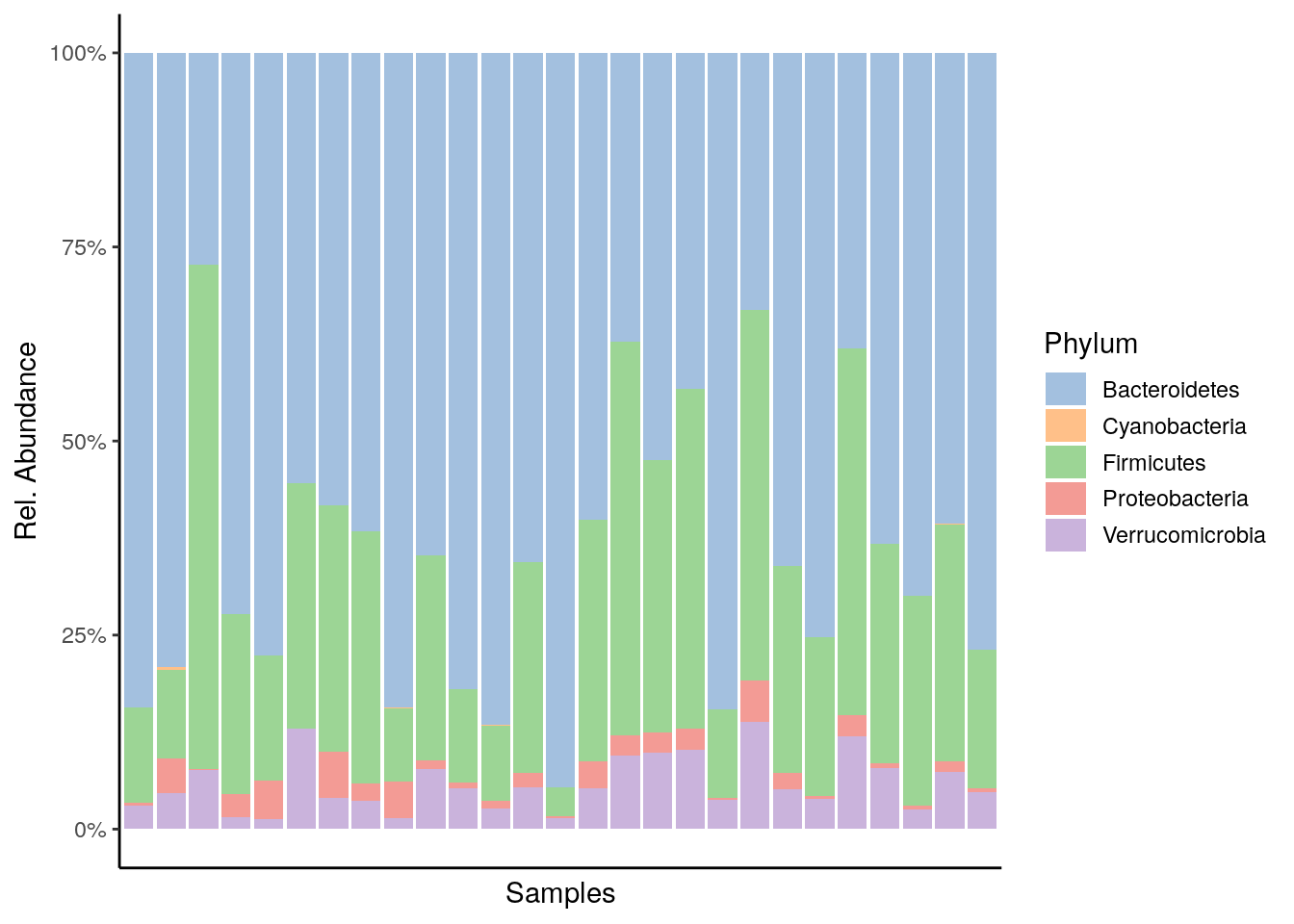 

Density plot shows the overall abundance distribution for a given taxonomic group. Let us check the relative abundance of Firmicutes across the sample collection. The density plot is a smoothened version of a standard histogram.

The plot shows peak abundances around 30 %.

# Subset data by taking only Firmicutes
tse_firmicutes <- tse_phylum["Firmicutes"]

# Gets the abundance table
abundance_firmicutes <- assay(tse_firmicutes, "relabundance")

# Creates a data frame object, where first column includes abundances
firmicutes_abund_df <- as.data.frame(t(abundance_firmicutes))
# Rename the first and only column
colnames(firmicutes_abund_df) <- "abund"

# Creates a plot. Parameters inside feom_density are optional. With 
# geom_density(bw=1000), it is possible to adjust bandwidth.
firmicutes_abund_plot <- ggplot(firmicutes_abund_df, aes(x = abund)) + 
  geom_density(color="darkred", fill="lightblue") + 
  labs(x = "Relative abundance", title = "Firmicutes") +
  theme_classic() + # Changes the background
  scale_x_continuous(label = scales::percent)

firmicutes_abund_plot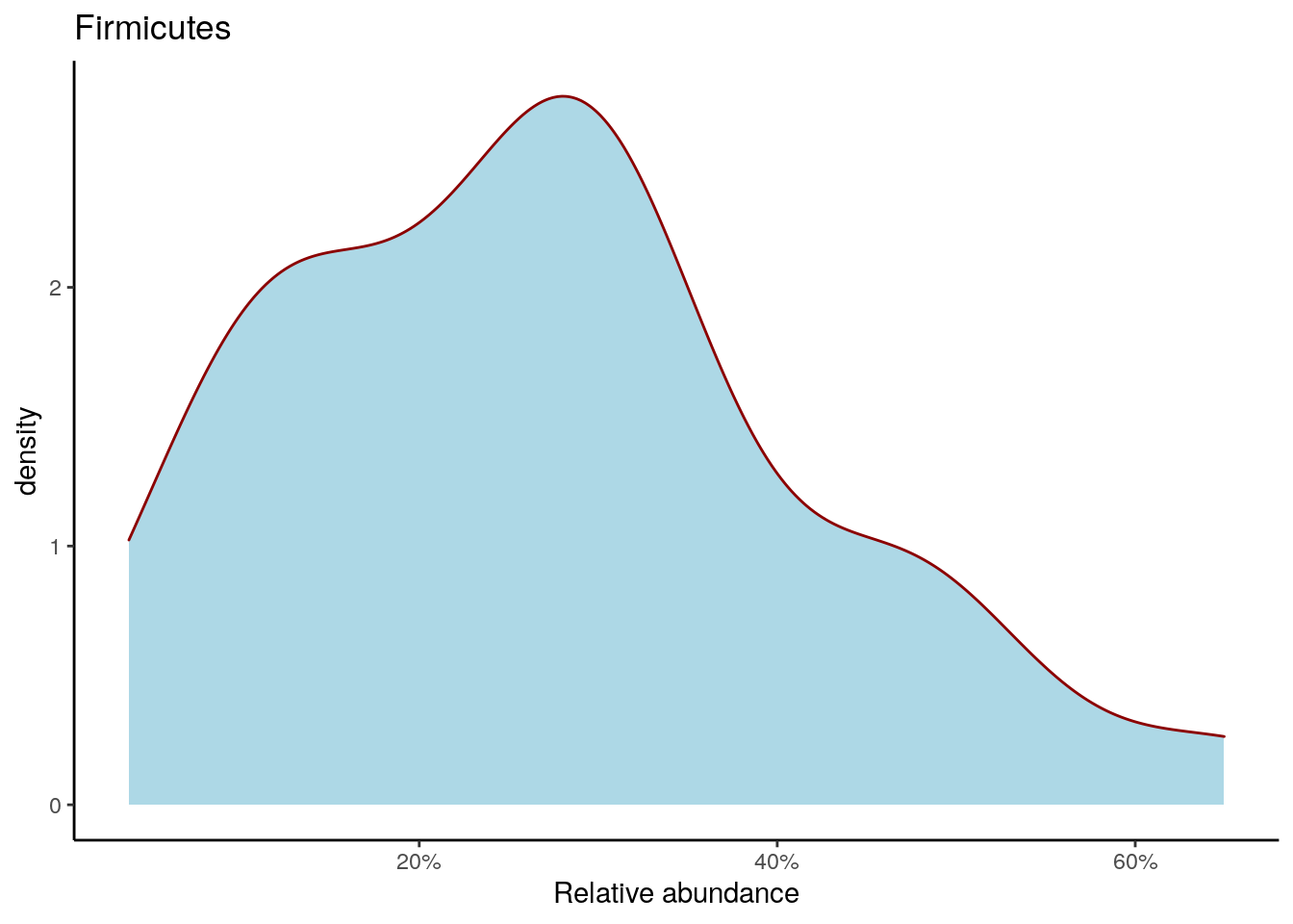

For more visualization options and examples, see the miaViz vignette.

6.3 Exercises (optional)

Explore some of the following questions on your own by following online examples. Prepare a reproducible report (Rmarkdown), and include the code that you use to import the data and generate the analyses.

• Abundance table Retrieve the taxonomic abundance table from the example data set (TSE object). Tip: check “assays” in data import section

• How many different samples and genus-level groups this phyloseq object has? Tips: see dim(), rowData()

• What is the maximum abundance of Akkermansia in this data set? Tip: aggregate the data to Genus level with agglomerateByRank, pick abundance assay, and check a given genus (row) in the assay

• Draw a histogram of library sizes (total number of reads per sample). Tip: Library size section in OMA. You can use the available function, or count the sum of reads per sample by using the colSums command applied on the abundance table. Check Vandeputte et al. 2017 for further discussion on the differences between absolute and relative quantification of microbial abundances.

• Taxonomy table Retrieve the taxonomy table and print out the first few lines of it with the R command head(). Investigate how many different phylum-level groups this phyloseq object has? Tips: rowData, taxonomicRanks in OMA.

• Sample metadata Retrieve sample metadata. How many patient groups this data set has? Draw a histogram of sample diversities. Tips: colData

• Subsetting Pick a subset of the data object including only ADHD individuals from Cohort 1. How many there are? Tips: subsetSamples

• Transformations The data contains read counts. We can convert these into relative abundances and other formats. Compare abundance of a given taxonomic group using the example data before and after the compositionality transformation (with a cross-plot, for instance). You can also compare the results to CLR-transformed data (see e.g. Gloor et al. 2017)

• Visual exploration Visualize the population distribution of abundances for certain taxonomic groups. Do the same for CLR-transformed abundances. Tip: assays, transformCounts

• Experiment with other data manipulation tools from OMA.

• Example solution: Solutions

## Loading required package: SummarizedExperiment

## Loading required package: MatrixGenerics

## Loading required package: matrixStats

## 
## Attaching package: 'MatrixGenerics'

## The following objects are masked from 'package:matrixStats':
## 
##     colAlls, colAnyNAs, colAnys, colAvgsPerRowSet, colCollapse,
##     colCounts, colCummaxs, colCummins, colCumprods, colCumsums,
##     colDiffs, colIQRDiffs, colIQRs, colLogSumExps, colMadDiffs,
##     colMads, colMaxs, colMeans2, colMedians, colMins, colOrderStats,
##     colProds, colQuantiles, colRanges, colRanks, colSdDiffs, colSds,
##     colSums2, colTabulates, colVarDiffs, colVars, colWeightedMads,
##     colWeightedMeans, colWeightedMedians, colWeightedSds,
##     colWeightedVars, rowAlls, rowAnyNAs, rowAnys, rowAvgsPerColSet,
##     rowCollapse, rowCounts, rowCummaxs, rowCummins, rowCumprods,
##     rowCumsums, rowDiffs, rowIQRDiffs, rowIQRs, rowLogSumExps,
##     rowMadDiffs, rowMads, rowMaxs, rowMeans2, rowMedians, rowMins,
##     rowOrderStats, rowProds, rowQuantiles, rowRanges, rowRanks,
##     rowSdDiffs, rowSds, rowSums2, rowTabulates, rowVarDiffs, rowVars,
##     rowWeightedMads, rowWeightedMeans, rowWeightedMedians,
##     rowWeightedSds, rowWeightedVars

## Loading required package: GenomicRanges

## Loading required package: stats4

## Loading required package: BiocGenerics

## 
## Attaching package: 'BiocGenerics'

## The following objects are masked from 'package:stats':
## 
##     IQR, mad, sd, var, xtabs

## The following objects are masked from 'package:base':
## 
##     anyDuplicated, append, as.data.frame, basename, cbind, colnames,
##     dirname, do.call, duplicated, eval, evalq, Filter, Find, get, grep,
##     grepl, intersect, is.unsorted, lapply, Map, mapply, match, mget,
##     order, paste, pmax, pmax.int, pmin, pmin.int, Position, rank,
##     rbind, Reduce, rownames, sapply, setdiff, sort, table, tapply,
##     union, unique, unsplit, which.max, which.min

## Loading required package: S4Vectors

## 
## Attaching package: 'S4Vectors'

## The following objects are masked from 'package:base':
## 
##     expand.grid, I, unname

## Loading required package: IRanges

## Loading required package: GenomeInfoDb

## Loading required package: Biobase

## Welcome to Bioconductor
## 
##     Vignettes contain introductory material; view with
##     'browseVignettes()'. To cite Bioconductor, see
##     'citation("Biobase")', and for packages 'citation("pkgname")'.

## 
## Attaching package: 'Biobase'

## The following object is masked from 'package:MatrixGenerics':
## 
##     rowMedians

## The following objects are masked from 'package:matrixStats':
## 
##     anyMissing, rowMedians

## Loading required package: SingleCellExperiment

## Loading required package: TreeSummarizedExperiment

## Loading required package: Biostrings

## Loading required package: XVector

## 
## Attaching package: 'Biostrings'

## The following object is masked from 'package:base':
## 
##     strsplit

## Loading required package: ggplot2

## Loading required package: ggraph

## 
## Attaching package: 'dplyr'

## The following objects are masked from 'package:Biostrings':
## 
##     collapse, intersect, setdiff, setequal, union

## The following object is masked from 'package:XVector':
## 
##     slice

## The following object is masked from 'package:Biobase':
## 
##     combine

## The following objects are masked from 'package:GenomicRanges':
## 
##     intersect, setdiff, union

## The following object is masked from 'package:GenomeInfoDb':
## 
##     intersect

## The following objects are masked from 'package:IRanges':
## 
##     collapse, desc, intersect, setdiff, slice, union

## The following objects are masked from 'package:S4Vectors':
## 
##     first, intersect, rename, setdiff, setequal, union

## The following objects are masked from 'package:BiocGenerics':
## 
##     combine, intersect, setdiff, union

## The following object is masked from 'package:matrixStats':
## 
##     count

## The following objects are masked from 'package:stats':
## 
##     filter, lag

## The following objects are masked from 'package:base':
## 
##     intersect, setdiff, setequal, union