Introduction
miaTime is a package in the mia family,
providing tools for time series manipulation using the TreeSummarizedExperiment
data container.
Installation
miaTime is hosted on Bioconductor, and can be installed
using via BiocManager.
BiocManager::install("miaTime")Divergence between time points
Divergence refers to the quantification of dissimilarity or difference between microbiome samples taken at different time points. This concept is crucial for tracking how microbial communities change or evolve over time, either in individuals or experimental conditions.
Types of divergence provided
miaTime provides several functions for calculating
divergences:
Baseline divergence: Measures the dissimilarity between each sample and a reference (typically the first time point) within a group (such as per subject).
Stepwise (rolling) divergence: Assesses the change between consecutive (or defined interval) time points by comparing each sample to the previous ith sample in the series.
The divergence is typically calculated using a beta diversity metric, such as Bray-Curtis dissimilarity, which quantifies how different two communities are in terms of their composition.
For rolling or stepwise divergences, the calculation measures how much the community shifts from one sampling point to the next.
Purpose
Quantifying divergence allows researchers to:
Track temporal instability or stability of the microbiome.
Compare change rates between individuals or treatments.
Identify significant shifts or stable periods in the microbiome composition.
Practical application
For example, in a human gut microbiome time series, calculating divergence helps determine how resistant the microbial ecosystem is to perturbations (such as antibiotics or diet changes) and how long it takes to return (if at all) to its original state.
Divergences can be calculated with *Divergence()
functions. In the example below, for each subject, we calculate the
divergence of their samples by comparing them to the first time
point.
data(hitchip1006)
tse <- hitchip1006

res <- getBaselineDivergence(
    tse, time.col = "time", group = "sample",
    name = c("baseline", "time_diff", "ref_samples"))
res |> head()
#> DataFrame with 6 rows and 3 columns
#>           baseline time_diff ref_samples
#>          <numeric> <numeric> <character>
#> Sample-1         0         0    Sample-1
#> Sample-2         0         0    Sample-2
#> Sample-3         0         0    Sample-3
#> Sample-4         0         0    Sample-4
#> Sample-5         0         0    Sample-5
#> Sample-6         0         0    Sample-6
A more convenient and preferred approach is to store the values
directly in colData using the add*Divergence()
functions. In the example below, we calculate stepwise divergences with
a lag of 1, meaning that for each sample, the divergence is calculated
by comparing it to the previous time point for the same subject.
tse <- addStepwiseDivergence(tse, time.col = "time")
colData(tse)
#> DataFrame with 1151 rows and 13 columns
#>                   age      sex nationality DNA_extraction_method  project
#>             <integer> <factor>    <factor>              <factor> <factor>
#> Sample-1           28   male            US                    NA        1
#> Sample-2           24   female          US                    NA        1
#> Sample-3           52   male            US                    NA        1
#> Sample-4           22   female          US                    NA        1
#> Sample-5           25   female          US                    NA        1
#> ...               ...      ...         ...                   ...      ...
#> Sample-1168        50   female Scandinavia                     r       40
#> Sample-1169        31   female Scandinavia                     r       40
#> Sample-1170        31   female Scandinavia                     r       40
#> Sample-1171        52   male   Scandinavia                     r       40
#> Sample-1172        52   male   Scandinavia                     r       40
#>             diversity   bmi_group  subject      time      sample divergence
#>             <numeric>    <factor> <factor> <numeric> <character>  <numeric>
#> Sample-1         5.76 severeobese        1         0    Sample-1         NA
#> Sample-2         6.06 obese              2         0    Sample-2         NA
#> Sample-3         5.50 lean               3         0    Sample-3         NA
#> Sample-4         5.87 underweight        4         0    Sample-4         NA
#> Sample-5         5.89 lean               5         0    Sample-5         NA
#> ...               ...         ...      ...       ...         ...        ...
#> Sample-1168      5.87 severeobese      244       8.1 Sample-1168   0.479394
#> Sample-1169      5.87 overweight       245       2.3 Sample-1169   0.356508
#> Sample-1170      5.92 overweight       245       8.2 Sample-1170   0.434298
#> Sample-1171      6.04 overweight       246       2.1 Sample-1171   0.403581
#> Sample-1172      5.74 overweight       246       7.9 Sample-1172   0.485427
#>             time_diff                             ref_samples
#>             <numeric>                                  <list>
#> Sample-1           NA                                      NA
#> Sample-2           NA                                      NA
#> Sample-3           NA                                      NA
#> Sample-4           NA                                      NA
#> Sample-5           NA                                      NA
#> ...               ...                                     ...
#> Sample-1168       0.2                             Sample-1172
#> Sample-1169       0.2                             Sample-1171
#> Sample-1170       0.1                 Sample-1127,Sample-1168
#> Sample-1171       0.7 Sample-1016,Sample-1022,Sample-1027,...
#> Sample-1172       0.1                             Sample-1162
Visualize time series
We can visualize time series data with miaViz. Below, we visualize 5 most abundant taxa.
library(miaViz)

p <- plotSeries(tse, assay.type = "counts",
    time.col = "time",
    features = getTop(tse, 5),
    colour.by = "rownames")
p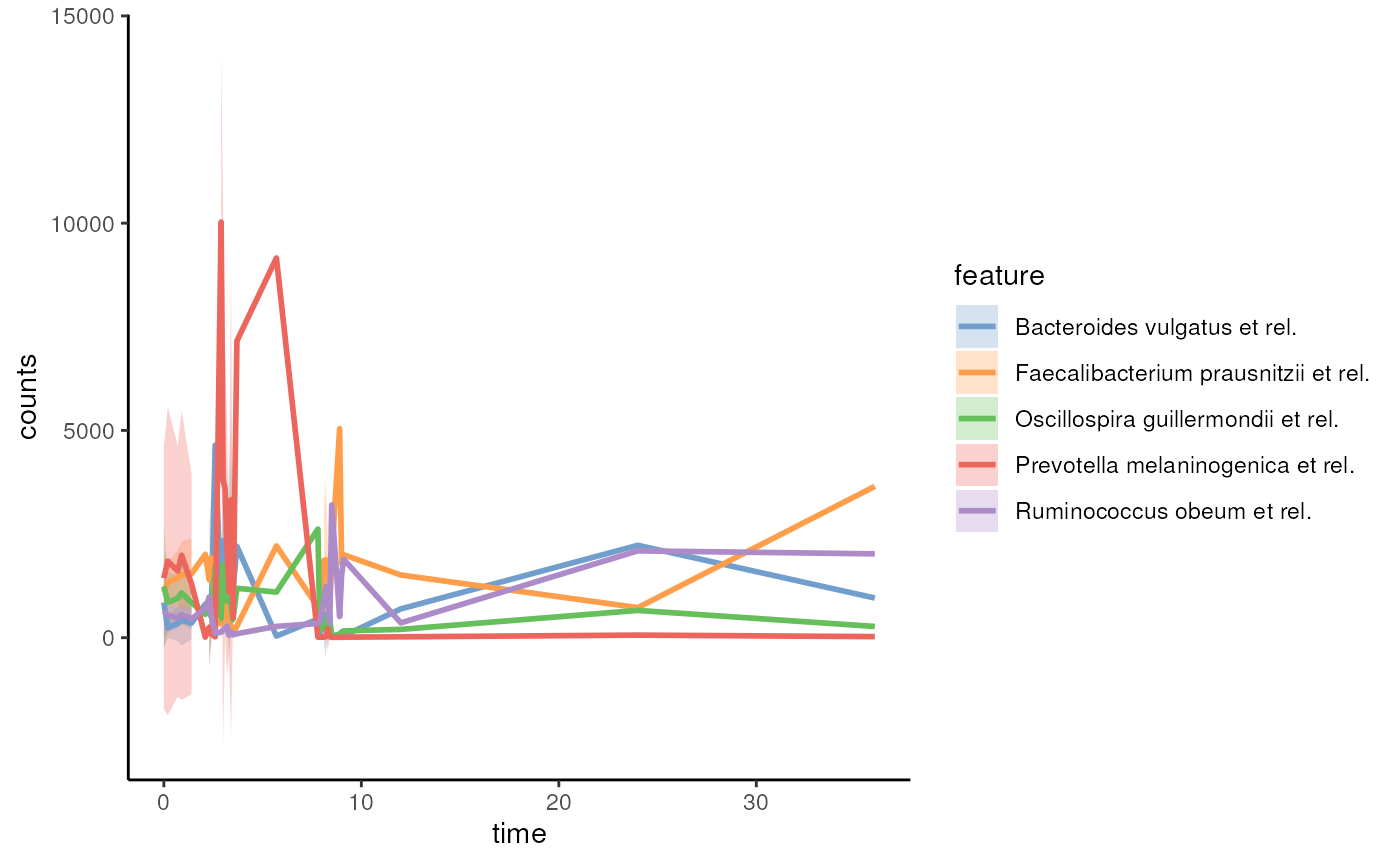
Session info
sessionInfo()
#> R version 4.5.1 (2025-06-13)
#> Platform: x86_64-pc-linux-gnu
#> Running under: Ubuntu 24.04.3 LTS
#>
#> Matrix products: default
#> BLAS:   /usr/lib/x86_64-linux-gnu/openblas-pthread/libblas.so.3
#> LAPACK: /usr/lib/x86_64-linux-gnu/openblas-pthread/libopenblasp-r0.3.26.so;  LAPACK version 3.12.0
#>
#> locale:
#>  [1] LC_CTYPE=en_US.UTF-8       LC_NUMERIC=C
#>  [3] LC_TIME=en_US.UTF-8        LC_COLLATE=en_US.UTF-8
#>  [5] LC_MONETARY=en_US.UTF-8    LC_MESSAGES=en_US.UTF-8
#>  [7] LC_PAPER=en_US.UTF-8       LC_NAME=C
#>  [9] LC_ADDRESS=C               LC_TELEPHONE=C
#> [11] LC_MEASUREMENT=en_US.UTF-8 LC_IDENTIFICATION=C
#>
#> time zone: UTC
#> tzcode source: system (glibc)
#>
#> attached base packages:
#> [1] stats4    stats     graphics  grDevices utils     datasets  methods
#> [8] base
#>
#> other attached packages:
#>  [1] miaViz_1.17.9                   ggraph_2.2.2
#>  [3] ggplot2_4.0.0                   miaTime_0.99.11
#>  [5] mia_1.17.9                      TreeSummarizedExperiment_2.17.1
#>  [7] Biostrings_2.77.2               XVector_0.49.1
#>  [9] SingleCellExperiment_1.31.1     MultiAssayExperiment_1.35.9
#> [11] SummarizedExperiment_1.39.2     Biobase_2.69.1
#> [13] GenomicRanges_1.61.5            Seqinfo_0.99.2
#> [15] IRanges_2.43.4                  S4Vectors_0.47.4
#> [17] BiocGenerics_0.55.1             generics_0.1.4
#> [19] MatrixGenerics_1.21.0           matrixStats_1.5.0
#> [21] knitr_1.50                      BiocStyle_2.37.1
#>
#> loaded via a namespace (and not attached):
#>   [1] RColorBrewer_1.1-3          jsonlite_2.0.0
#>   [3] magrittr_2.0.4              estimability_1.5.1
#>   [5] ggbeeswarm_0.7.2            farver_2.1.2
#>   [7] rmarkdown_2.30              fs_1.6.6
#>   [9] ragg_1.5.0                  vctrs_0.6.5
#>  [11] memoise_2.0.1               DelayedMatrixStats_1.31.0
#>  [13] ggtree_3.99.0               htmltools_0.5.8.1
#>  [15] S4Arrays_1.9.1              BiocBaseUtils_1.11.2
#>  [17] BiocNeighbors_2.3.1         janeaustenr_1.0.0
#>  [19] cellranger_1.1.0            gridGraphics_0.5-1
#>  [21] SparseArray_1.9.1           sass_0.4.10
#>  [23] parallelly_1.45.1           bslib_0.9.0
#>  [25] tokenizers_0.3.0            htmlwidgets_1.6.4
#>  [27] desc_1.4.3                  plyr_1.8.9
#>  [29] DECIPHER_3.5.0              emmeans_1.11.2-8
#>  [31] cachem_1.1.0                uuid_1.2-1
#>  [33] igraph_2.1.4                lifecycle_1.0.4
#>  [35] pkgconfig_2.0.3             rsvd_1.0.5
#>  [37] Matrix_1.7-4                R6_2.6.1
#>  [39] fastmap_1.2.0               tidytext_0.4.3
#>  [41] aplot_0.2.9                 digest_0.6.37
#>  [43] ggnewscale_0.5.2            patchwork_1.3.2
#>  [45] scater_1.37.0               irlba_2.3.5.1
#>  [47] SnowballC_0.7.1             textshaping_1.0.3
#>  [49] vegan_2.7-1                 beachmat_2.25.5
#>  [51] labeling_0.4.3              polyclip_1.10-7
#>  [53] abind_1.4-8                 mgcv_1.9-3
#>  [55] compiler_4.5.1              withr_3.0.2
#>  [57] S7_0.2.0                    BiocParallel_1.43.4
#>  [59] viridis_0.6.5               DBI_1.2.3
#>  [61] ggforce_0.5.0               MASS_7.3-65
#>  [63] rappdirs_0.3.3              DelayedArray_0.35.3
#>  [65] bluster_1.19.0              permute_0.9-8
#>  [67] tools_4.5.1                 vipor_0.4.7
#>  [69] beeswarm_0.4.0              ape_5.8-1
#>  [71] glue_1.8.0                  nlme_3.1-168
#>  [73] gridtext_0.1.5              grid_4.5.1
#>  [75] cluster_2.1.8.1             reshape2_1.4.4
#>  [77] gtable_0.3.6                fillpattern_1.0.2
#>  [79] tzdb_0.5.0                  tidyr_1.3.1
#>  [81] hms_1.1.3                   tidygraph_1.3.1
#>  [83] BiocSingular_1.25.0         ScaledMatrix_1.17.0
#>  [85] xml2_1.4.0                  ggrepel_0.9.6
#>  [87] pillar_1.11.1               stringr_1.5.2
#>  [89] yulab.utils_0.2.1           splines_4.5.1
#>  [91] tweenr_2.0.3                dplyr_1.1.4
#>  [93] ggtext_0.1.2                treeio_1.33.0
#>  [95] lattice_0.22-7              tidyselect_1.2.1
#>  [97] DirichletMultinomial_1.51.0 scuttle_1.19.0
#>  [99] gridExtra_2.3               bookdown_0.44
#> [101] xfun_0.53                   graphlayouts_1.2.2
#> [103] rbiom_2.2.1                 stringi_1.8.7
#> [105] ggfun_0.2.0                 lazyeval_0.2.2
#> [107] yaml_2.3.10                 evaluate_1.0.5
#> [109] codetools_0.2-20            tibble_3.3.0
#> [111] BiocManager_1.30.26         ggplotify_0.1.3
#> [113] cli_3.6.5                   xtable_1.8-4
#> [115] systemfonts_1.3.0           jquerylib_0.1.4
#> [117] Rcpp_1.1.0                  readxl_1.4.5
#> [119] parallel_4.5.1              pkgdown_2.1.3
#> [121] readr_2.1.5                 sparseMatrixStats_1.21.0
#> [123] decontam_1.29.0             viridisLite_0.4.2
#> [125] mvtnorm_1.3-3               slam_0.1-55
#> [127] tidytree_0.4.6              ggiraph_0.9.1
#> [129] scales_1.4.0                purrr_1.1.0
#> [131] crayon_1.5.3                rlang_1.1.6