Creates a two-dimensional ordination plot from a reduced dimension result
stored in a
SingleCellExperiment
object. Samples can be coloured, filled, shaped, sized, grouped or faceted
using sample metadata or feature abundances, and additional graphical
elements such as confidence ellipses, centroids, vectors and density
estimates can be added.
plotOrdination(x, ...)

# S4 method for class 'SingleCellExperiment'
plotOrdination(x, dimred, ...)
Arguments
- x
a
SummarizedExperimentobject.- ...
Additional parameters for plotting.
ncomponents:integer vectorof length 2 orinteger scalar. Specifies which ordination components are plotted. If a scalar is provided, the first two components are used. (Default:2L)colour.by:NULLorcharacter scalar. Specifies a variable fromcolData(x)or a feature fromrownames(x)used to colour observations. Feature abundances are taken fromassay.type. (Default:NULL)fill.by:NULLorcharacter scalar. Specifies a variable fromcolData(x)or a feature fromrownames(x)used to fill observations or ellipses. Feature abundances are taken fromassay.type. Cannot be used together withadd.density = TRUE. (Default:NULL)shape.by:NULLorcharacter scalar. Specifies a categorical variable fromcolData(x)used for point shapes. (Default:NULL)size.by:NULLorcharacter scalar. Specifies a variable fromcolData(x)used for point sizes. (Default:NULL)group.by:NULLorcharacter scalar. Specifies a categorical variable fromcolData(x)used for grouping when drawing ellipses, centroids and centroid vectors. (Default:NULL)linetype.by:NULLorcharacter scalar. Specifies a categorical variable fromcolData(x)used for ellipse line types. (Default:NULL)pair.by:NULLorcharacter scalar. Specifies a variable fromcolData(x)identifying observations that should be connected by lines. (Default:NULL)sort.by:NULLorcharacter scalar. Specifies a variable fromcolData(x)used to order observations before drawing connecting lines. (Default:NULL)facet.by:NULLorcharacter scalar. Specifies a categorical variable fromcolData(x)used to split the plot into facets. (Default:NULL)assay.type:character scalar. Name of the assay used whencolour.byorfill.byspecifies a feature. (Default:"counts")add.points:logical scalar. Whether to draw sample points. (Default:TRUE)add.ellipse:logical scalar. Whether to draw confidence ellipses around groups. (Default:FALSE)add.density:logical scalar. Whether to draw a two-dimensional density estimate in the background. (Default:FALSE)add.centroids:logical scalar. Whether to draw group centroids. (Default:FALSE)add.centroids.lines:logical scalar. Whether to connect observations to their group centroids. (Default:FALSE)add.vectors:logical scalar. Whether to draw vectors from the global centroid to group centroids. (Default:FALSE)add.rotation:logical scalar. Whether to draw rotation (species score) coordinates if available in the ordination result. (Default:add.species)add.species:logical scalar. Alias foradd.rotation. (Default:FALSE)add.expl.var:logical scalar. Whether to append the percentage of explained variance to the axis labels when available. (Default:FALSE)scales:character scalar. Scaling used for faceted plots. Passed toggplot2::facet_wrap(). (Default:"fixed")xlab,ylab:character scalar. Axis labels. Defaults to the ordination component names.panel.by.eigen:logical scalar. Whether to scale the panel aspect ratio according to the eigenvalues of the ordination when available. (Default:TRUE)point.shape: Shape used for points. (Default:19)point.alpha:numeric scalar. Transparency of points. Must be between 0 and 1. (Default:0.4)ellipse.alpha:numeric scalar. Transparency of ellipse fills. Must be between 0 and 1. (Default:0.2)ellipse.linewidth:numeric scalar. Line width of ellipse borders. (Default:0.5or0whenfill.byis specified.)ellipse.linetype: Integer specifying the ellipse line type. (Default:1)confidence.level:numeric scalar. Confidence level used for ellipse calculation. Must be between 0 and 1. (Default:0.95)adjust:numeric scalar. Multiplicative adjustment for the bandwidth used in the background density estimate. (Default:1)
- dimred
character scalar. Name of the reduced dimension result stored inreducedDim(x)to visualize.
Value
A ggplot2 object.
Details
This function provides a unified interface for visualizing ordination methods
such as PCA, PCoA, MDS, t-SNE, UMAP, RDA and CCA. The plotted coordinates are
retrieved from a reduced dimension result stored in
reducedDim(x).
See also
Examples
data("Tito2024QMP")
tse <- Tito2024QMP
# Compute relative abundances and an MDS ordination
tse <- transformAssay(tse, method = "relabundance")
tse <- addMDS(tse, assay.type = "relabundance", method = "bray", ncomponents = 50)
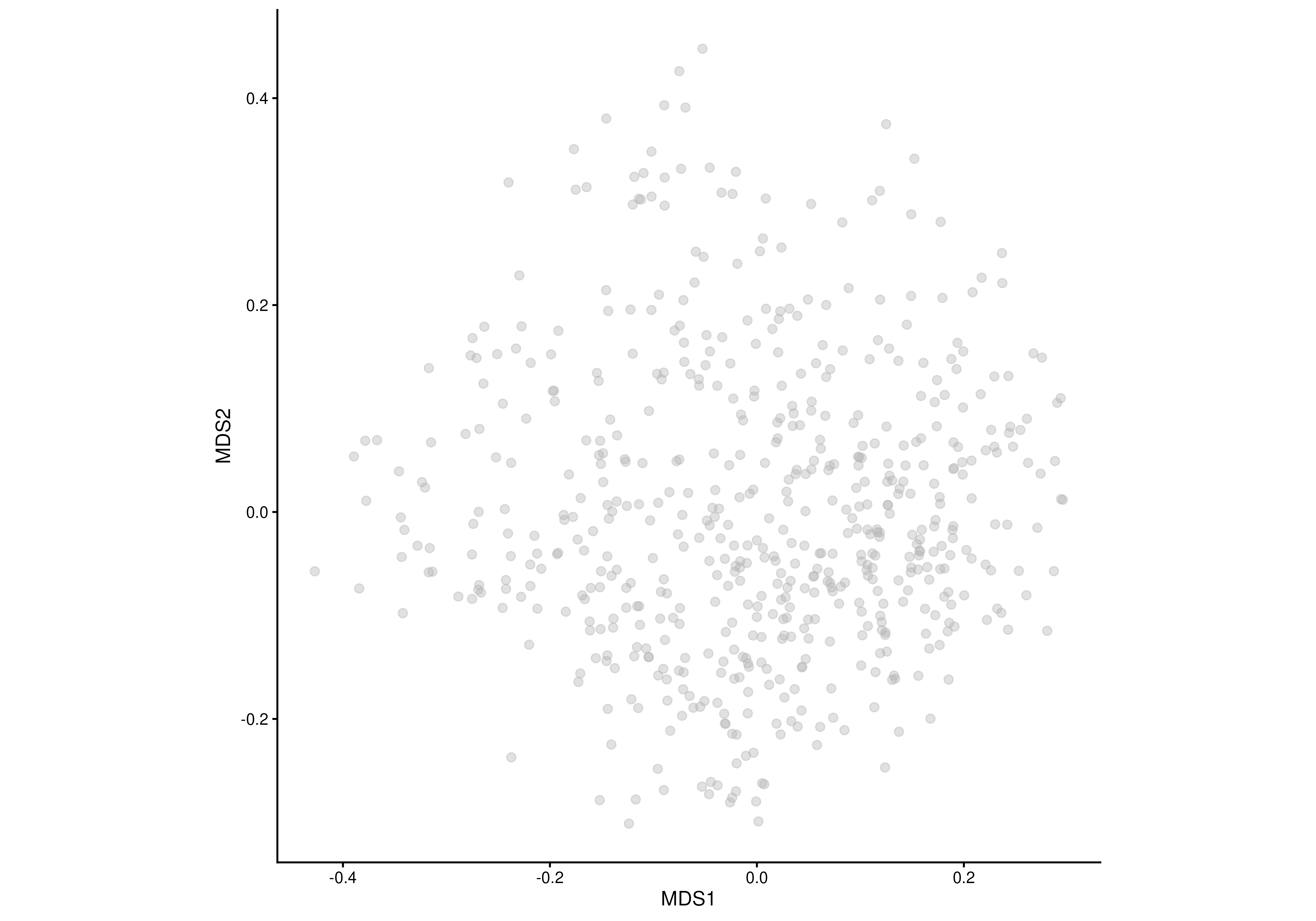
# Basic ordination plot
plotOrdination(tse, "MDS")
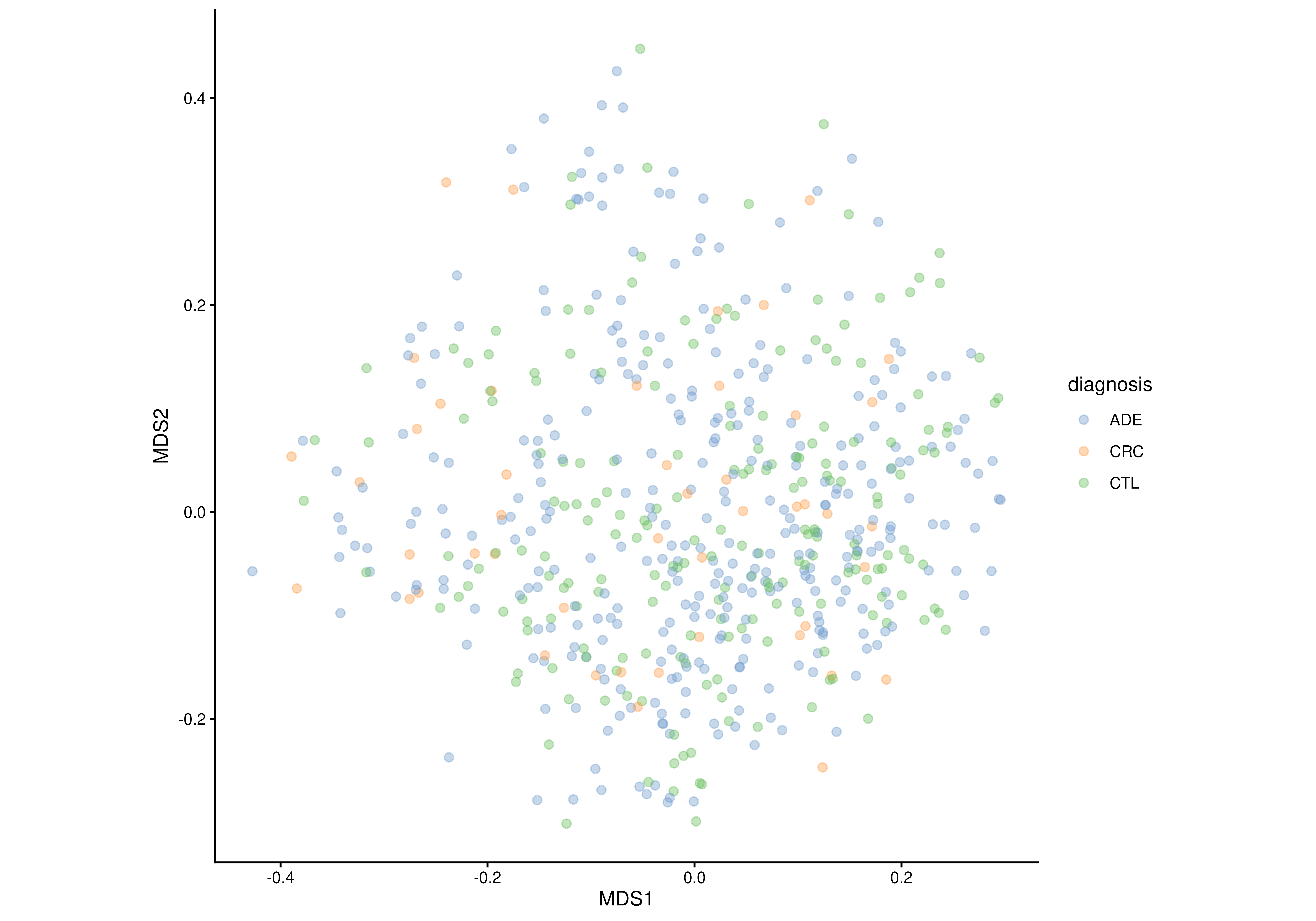
 # Colour samples by a sample-level variable
plotOrdination(tse, "MDS", colour.by = "diagnosis")
# Colour samples by a sample-level variable
plotOrdination(tse, "MDS", colour.by = "diagnosis")
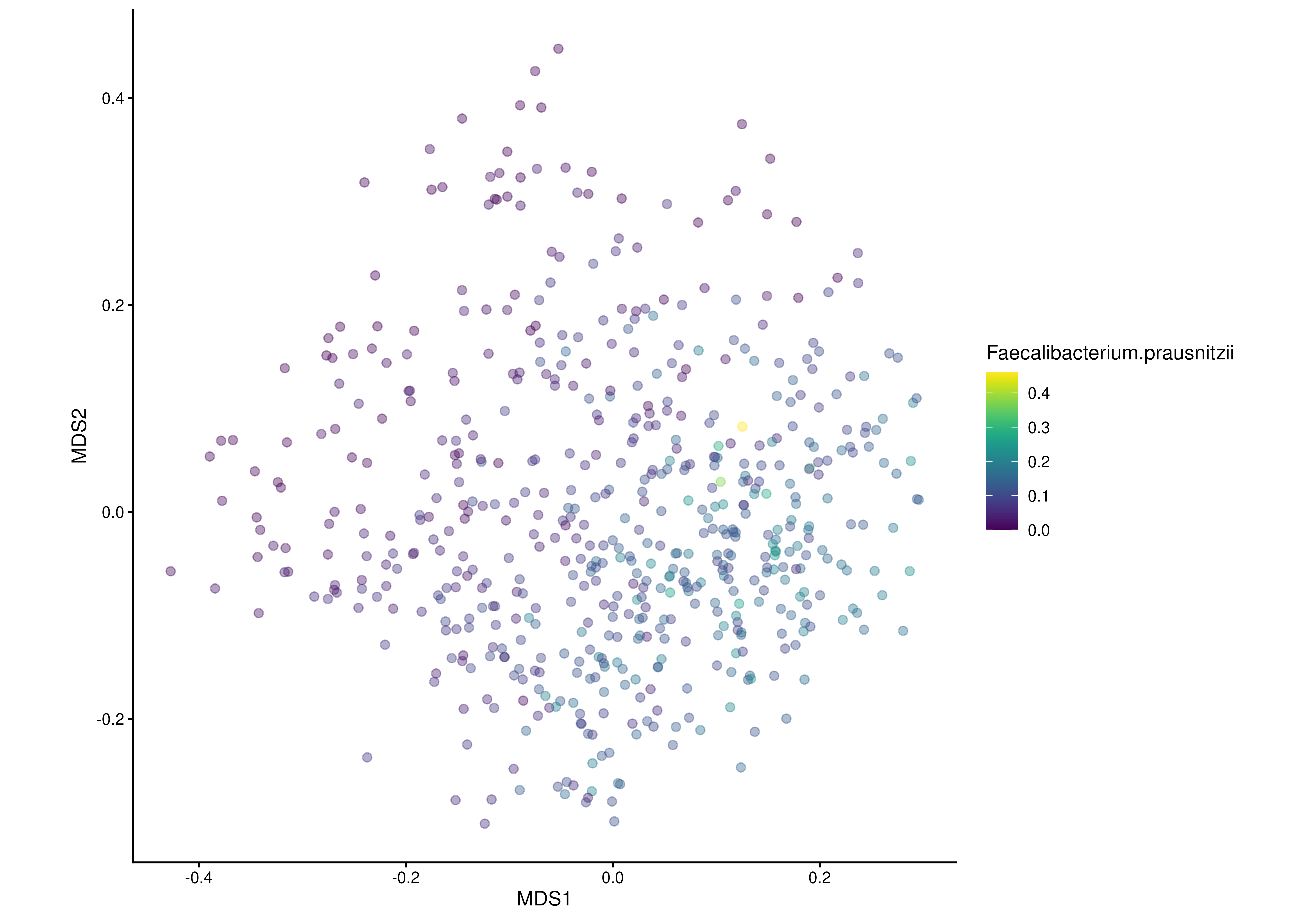
 # Colour samples by the abundance of a single feature
plotOrdination(
tse, "MDS",
colour.by = rownames(tse)[1],
assay.type = "relabundance")
# Colour samples by the abundance of a single feature
plotOrdination(
tse, "MDS",
colour.by = rownames(tse)[1],
assay.type = "relabundance")
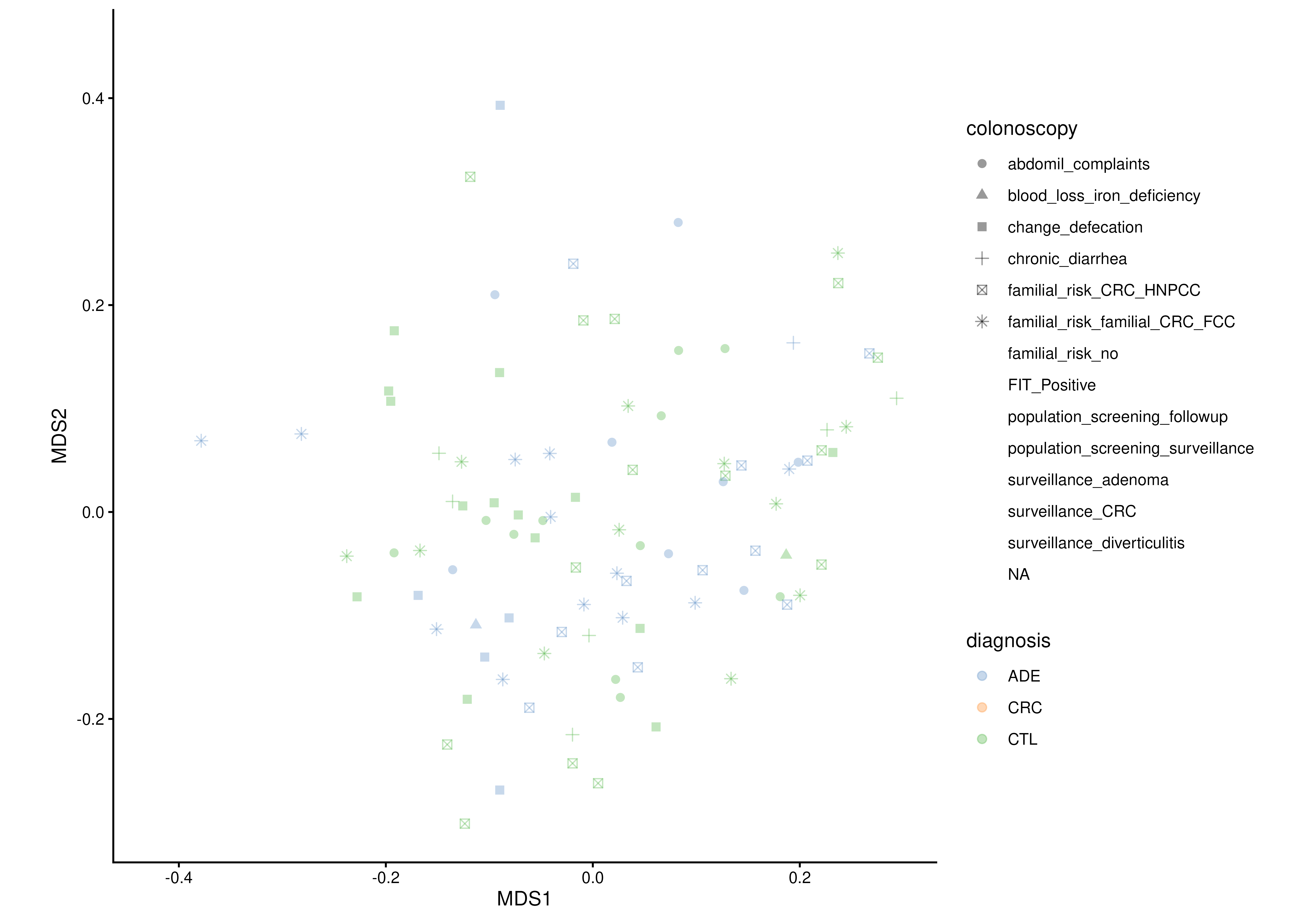
 # Use multiple aesthetics simultaneously
plotOrdination(
tse, "MDS",
colour.by = "diagnosis",
shape.by = "colonoscopy"
)
#> Warning: The shape palette can deal with a maximum of 6 discrete values because more
#> than 6 becomes difficult to discriminate
#> ℹ you have requested 13 values. Consider specifying shapes manually if you need
#> that many of them.
#> Warning: Removed 493 rows containing missing values or values outside the scale range
#> (`geom_point()`).
# Use multiple aesthetics simultaneously
plotOrdination(
tse, "MDS",
colour.by = "diagnosis",
shape.by = "colonoscopy"
)
#> Warning: The shape palette can deal with a maximum of 6 discrete values because more
#> than 6 becomes difficult to discriminate
#> ℹ you have requested 13 values. Consider specifying shapes manually if you need
#> that many of them.
#> Warning: Removed 493 rows containing missing values or values outside the scale range
#> (`geom_point()`).
 # Add confidence ellipses
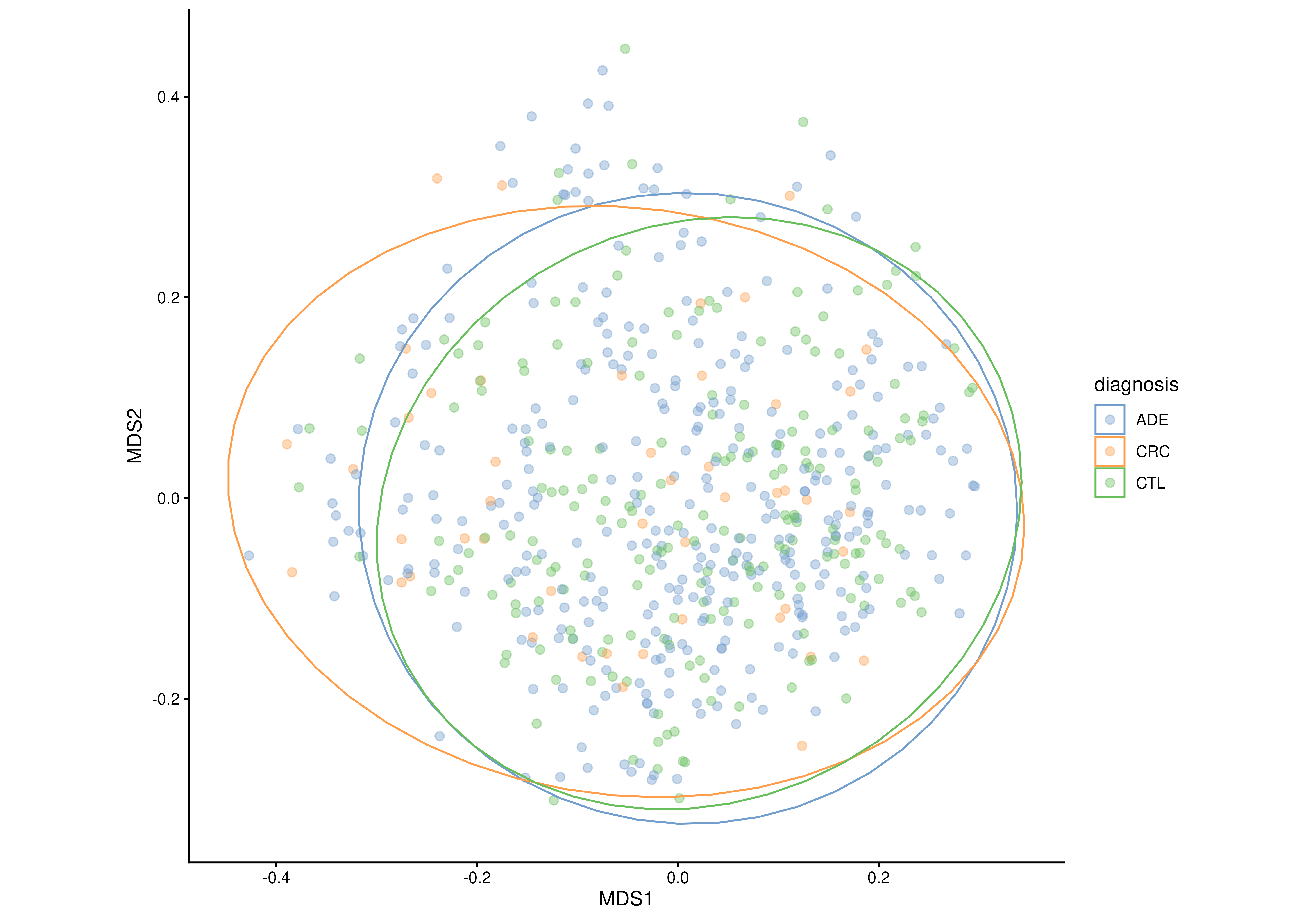
plotOrdination(
tse, "MDS",
colour.by = "diagnosis",
group.by = "diagnosis",
add.ellipse = TRUE
)
# Add confidence ellipses
plotOrdination(
tse, "MDS",
colour.by = "diagnosis",
group.by = "diagnosis",
add.ellipse = TRUE
)
 # Fill ellipses instead of colouring them
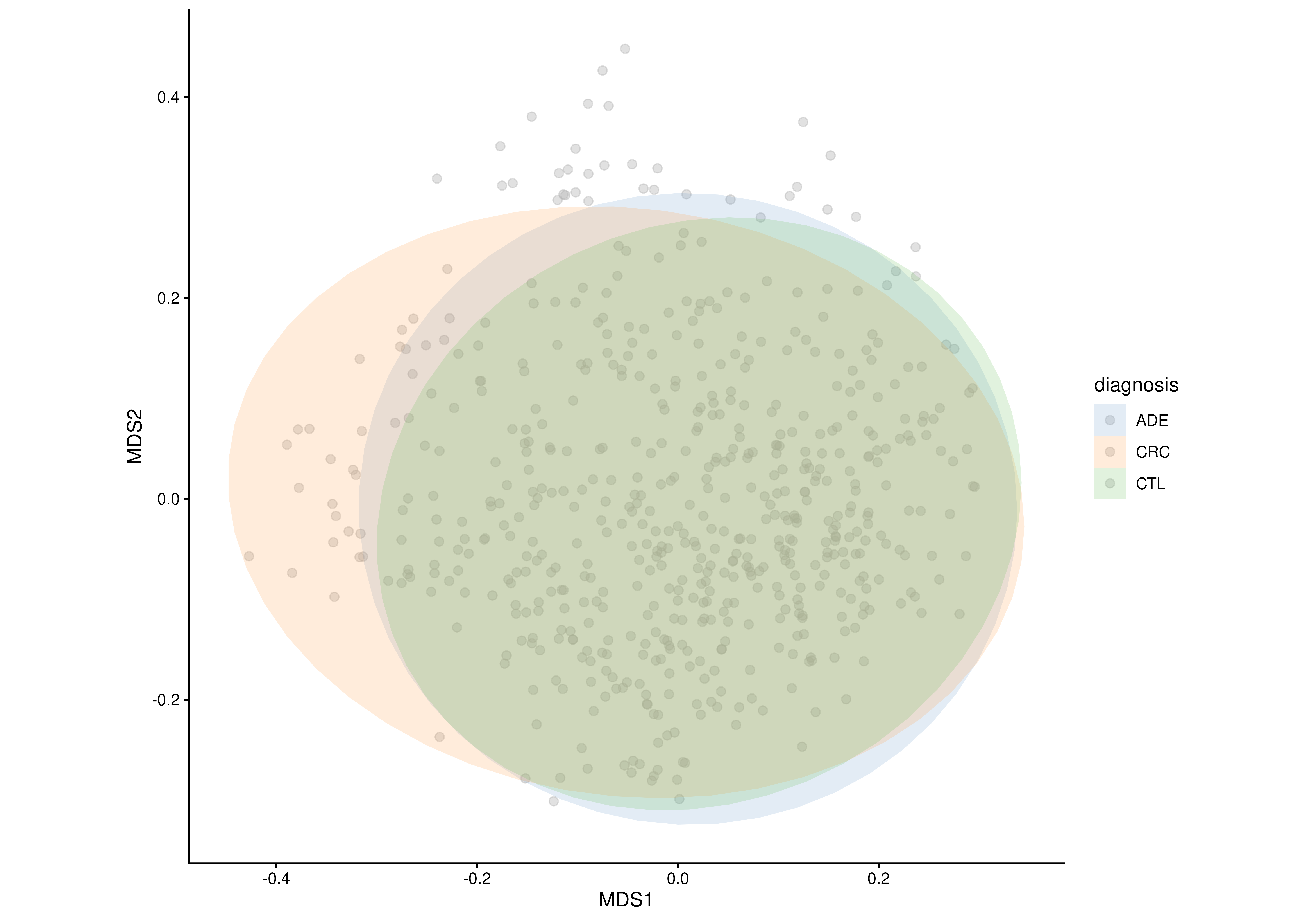
plotOrdination(
tse, "MDS",
fill.by = "diagnosis",
group.by = "diagnosis",
add.ellipse = TRUE
)
# Fill ellipses instead of colouring them
plotOrdination(
tse, "MDS",
fill.by = "diagnosis",
group.by = "diagnosis",
add.ellipse = TRUE
)
 # Show explained variance in the axis labels
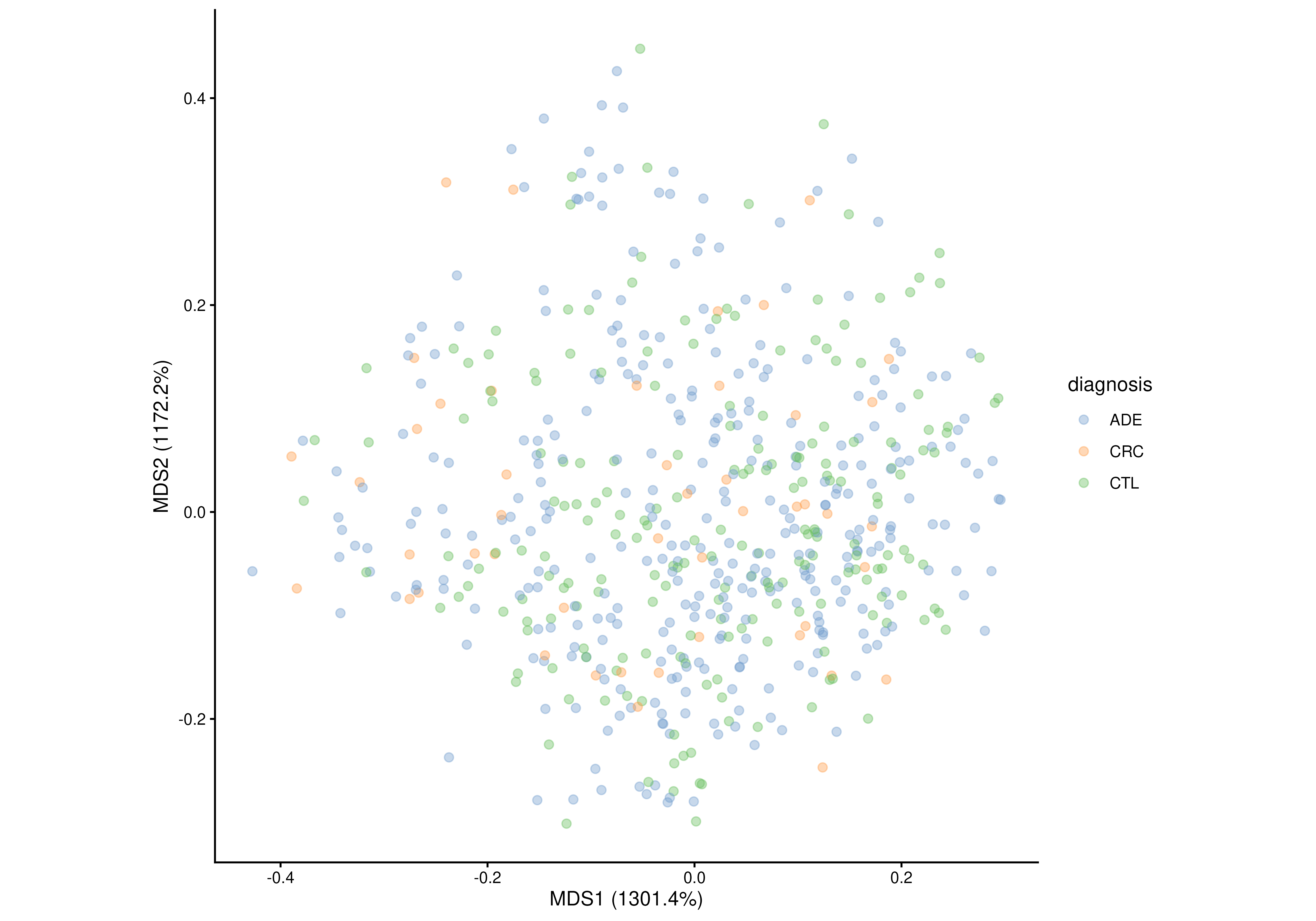
plotOrdination(
tse, "MDS",
colour.by = "diagnosis",
add.expl.var = TRUE
)
# Show explained variance in the axis labels
plotOrdination(
tse, "MDS",
colour.by = "diagnosis",
add.expl.var = TRUE
)
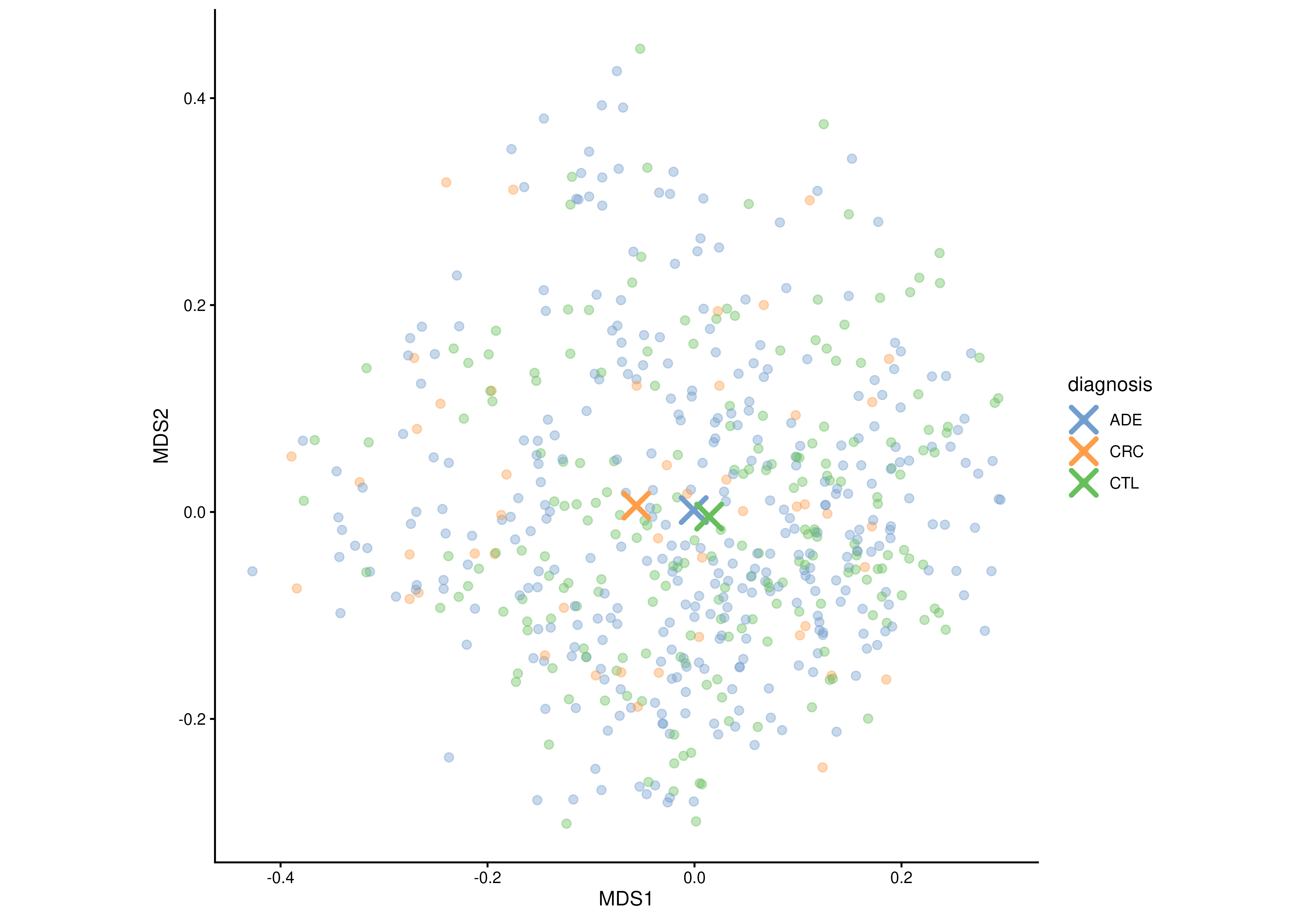
 # Add group centroids
plotOrdination(
tse, "MDS",
colour.by = "diagnosis",
group.by = "diagnosis",
add.centroids = TRUE
)
# Add group centroids
plotOrdination(
tse, "MDS",
colour.by = "diagnosis",
group.by = "diagnosis",
add.centroids = TRUE
)
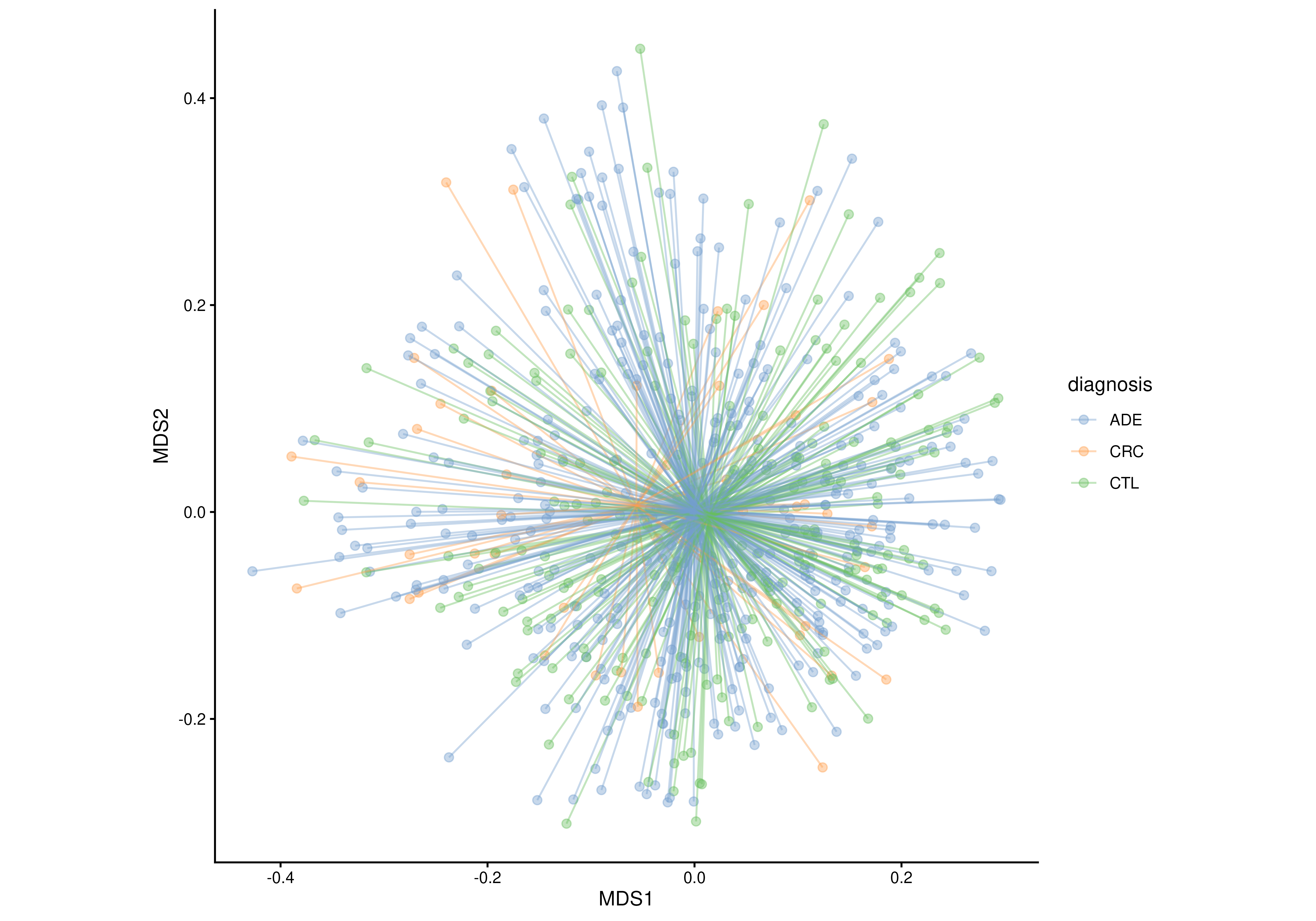
 # Connect samples to their group centroids
plotOrdination(
tse, "MDS",
colour.by = "diagnosis",
group.by = "diagnosis",
add.centroids.lines = TRUE
)
# Connect samples to their group centroids
plotOrdination(
tse, "MDS",
colour.by = "diagnosis",
group.by = "diagnosis",
add.centroids.lines = TRUE
)
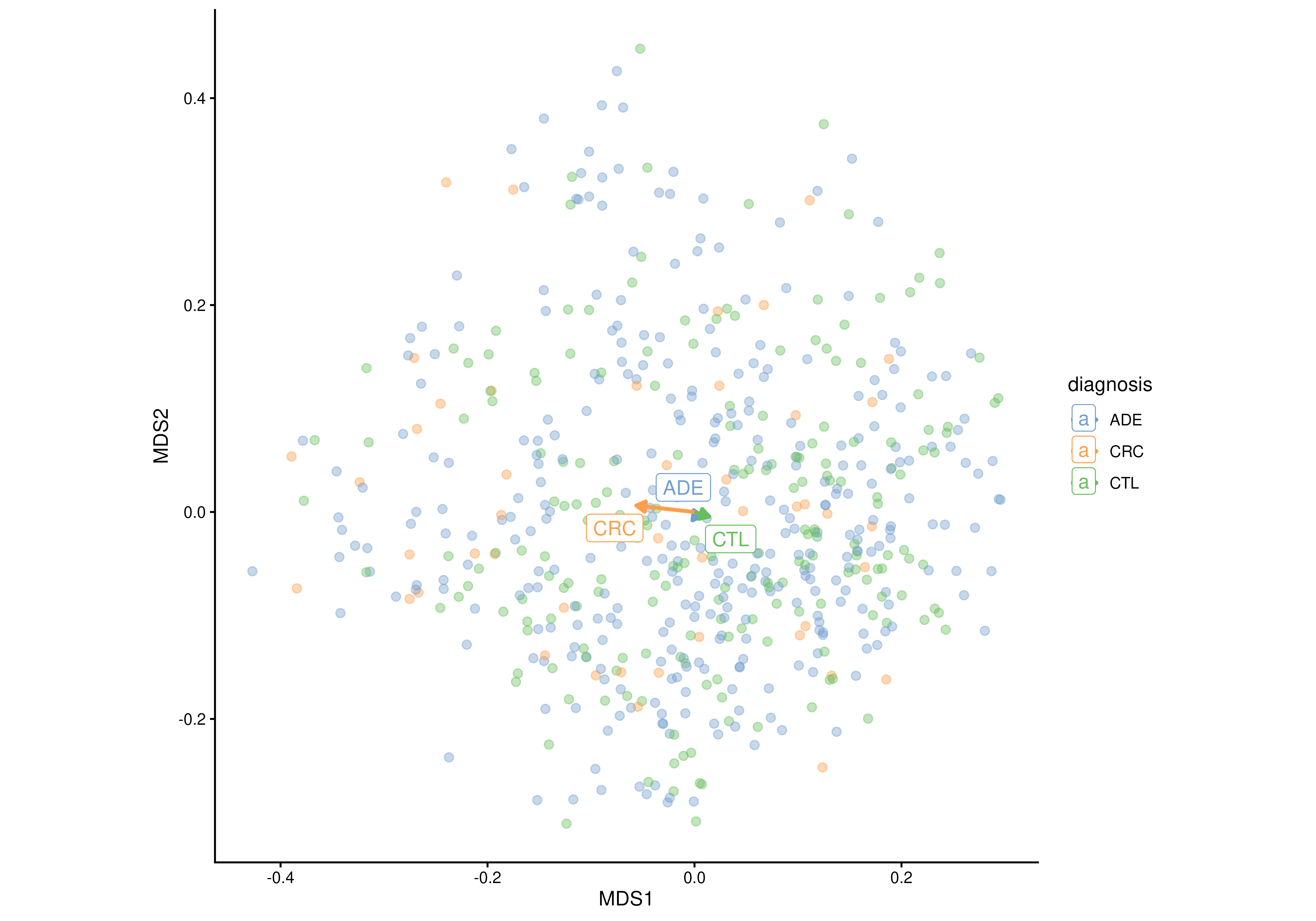
 # Show vectors from the global centroid to each group centroid
plotOrdination(
tse, "MDS",
colour.by = "diagnosis",
group.by = "diagnosis",
add.vectors = TRUE
)
#> Warning: Using `size` aesthetic for lines was deprecated in ggplot2 3.4.0.
#> ℹ Please use `linewidth` instead.
#> ℹ The deprecated feature was likely used in the miaViz package.
#> Please report the issue at <https://github.com/microbiome/miaViz/issues>.
# Show vectors from the global centroid to each group centroid
plotOrdination(
tse, "MDS",
colour.by = "diagnosis",
group.by = "diagnosis",
add.vectors = TRUE
)
#> Warning: Using `size` aesthetic for lines was deprecated in ggplot2 3.4.0.
#> ℹ Please use `linewidth` instead.
#> ℹ The deprecated feature was likely used in the miaViz package.
#> Please report the issue at <https://github.com/microbiome/miaViz/issues>.
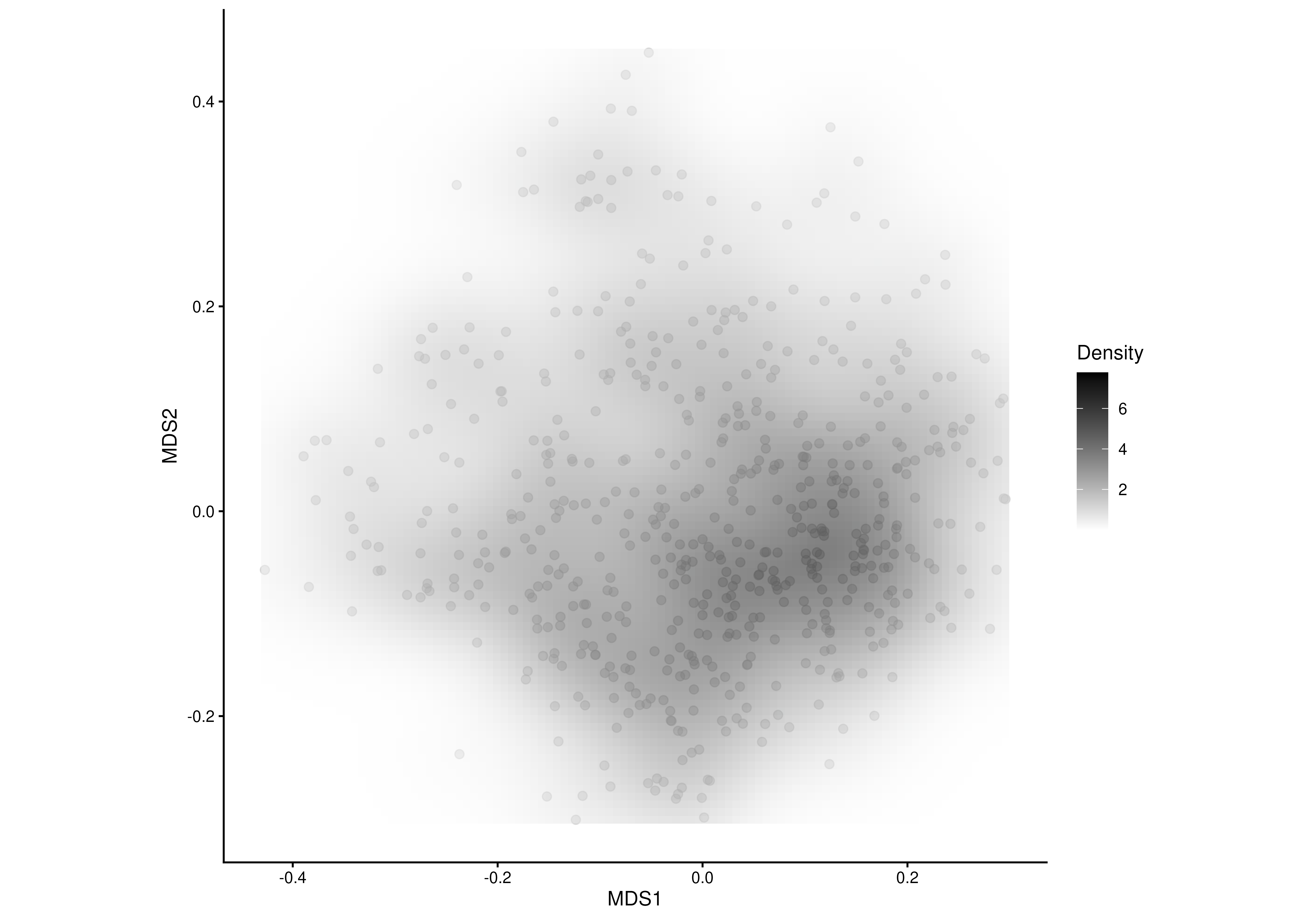
 # Draw a background density estimate
plotOrdination(
tse, "MDS",
add.density = TRUE
)
# Draw a background density estimate
plotOrdination(
tse, "MDS",
add.density = TRUE
)
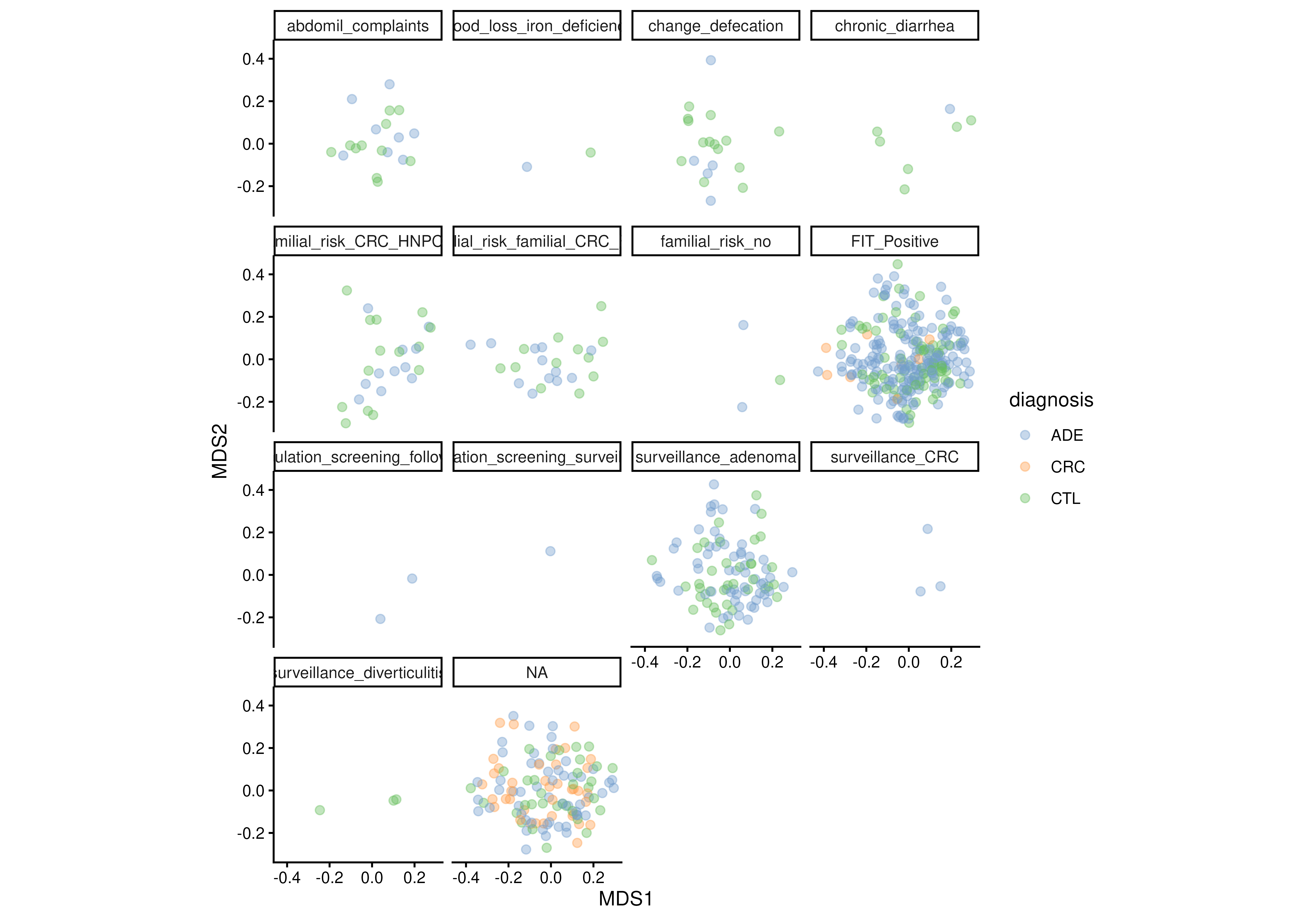
 # Split the plot into facets
plotOrdination(
tse, "MDS",
colour.by = "diagnosis",
facet.by = "colonoscopy"
)
# Split the plot into facets
plotOrdination(
tse, "MDS",
colour.by = "diagnosis",
facet.by = "colonoscopy"
)
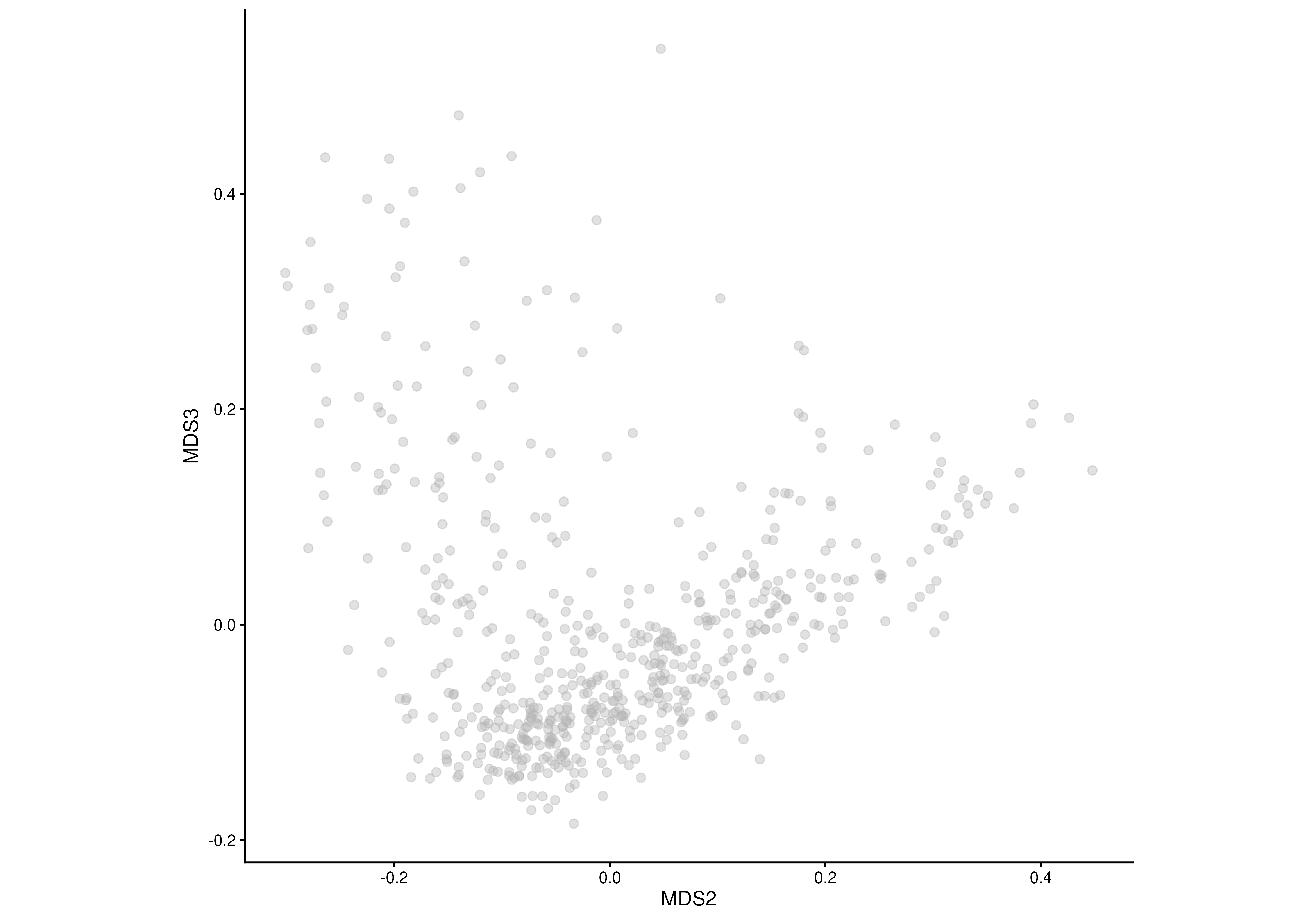
 # Plot different ordination components
plotOrdination(
tse, "MDS",
ncomponents = c(2, 3)
)
# Plot different ordination components
plotOrdination(
tse, "MDS",
ncomponents = c(2, 3)
)
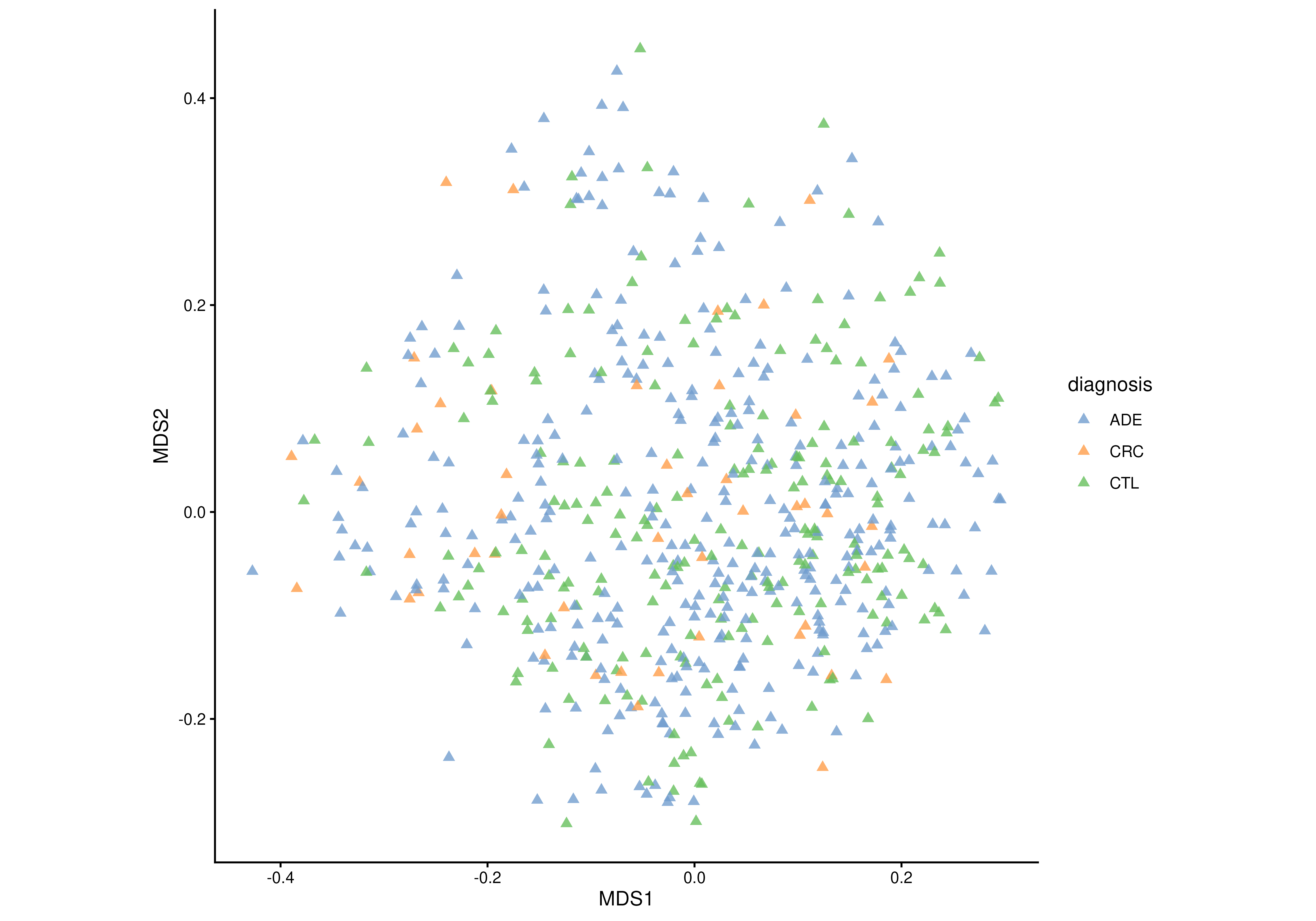
 # Customize point appearance
plotOrdination(
tse, "MDS",
colour.by = "diagnosis",
point.shape = 17,
point.alpha = 0.8
)
# Customize point appearance
plotOrdination(
tse, "MDS",
colour.by = "diagnosis",
point.shape = 17,
point.alpha = 0.8
)