Minimal gut bioreactor examples

Minimal gut microbiome

Dense samples of the minimal gut microbiome. In the initial hours, MDb-MM was grown under batch condition and 24 h onwards, continuous feeding of media with pulse feeding cycles. This information is stored in the colData.

library(miaTime)
data(minimalgut)
tse <- minimalgut

# Quick check of number of samples 
table(tse[["StudyIdentifier"]], tse[["condition_1"]])
#>               
#>                batch_carbs DoS pulse Overnight
#>   Bioreactor A           4        38        19
#>   Bioreactor B           4        38        19
#>   Bioreactor C           4        38        19

Visualize samples available for each of the bioreactors. This allows to identify if there are any missing samples for specific times.

library(ggplot2)

colData(tse) |>
    ggplot() +
    geom_tile(
        aes(x = as.factor(Time.hr), y = StudyIdentifier, fill = condition_1))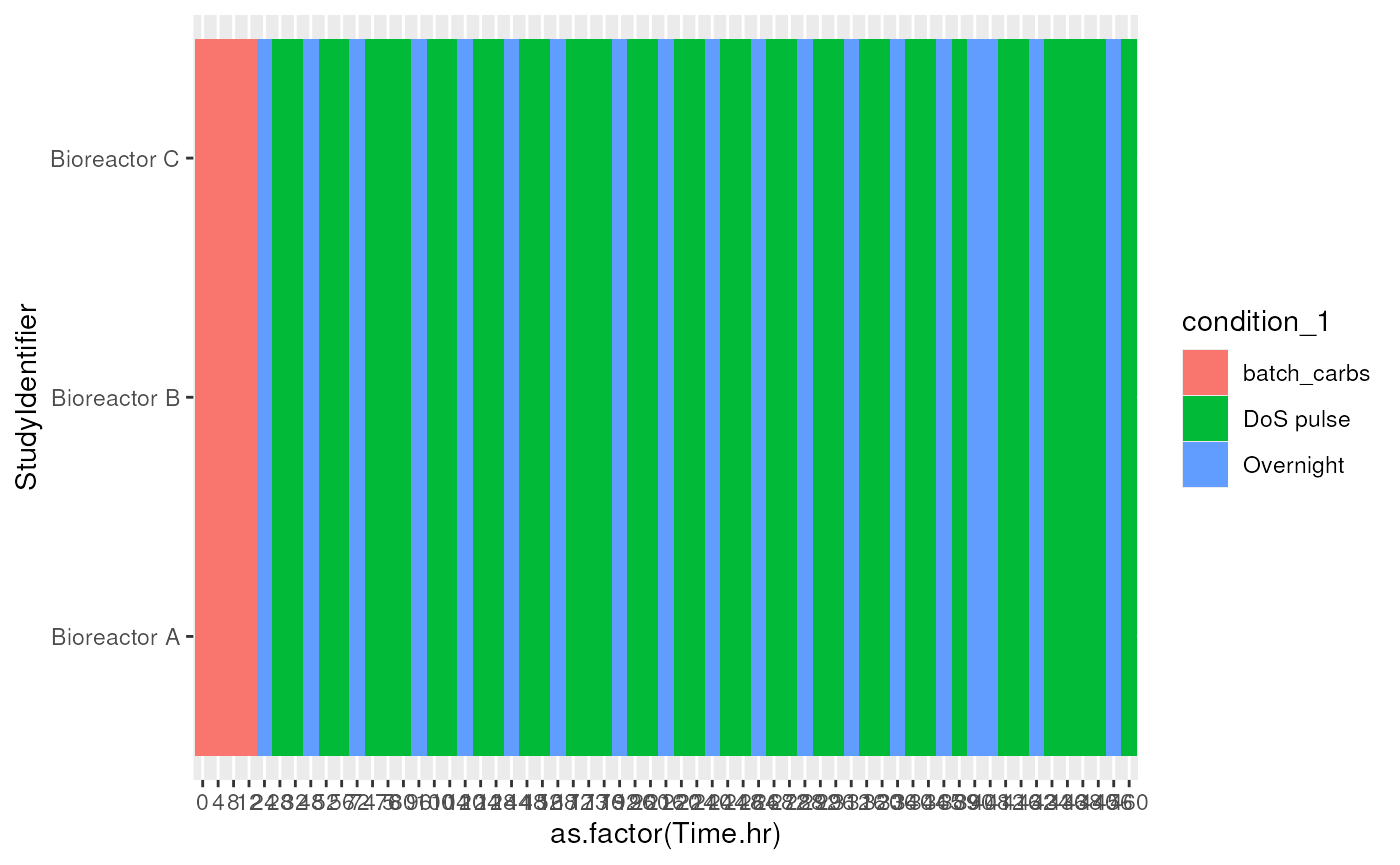

Community dynamics

The minimalgut dataset, mucus-diet based minimal microbiome (MDbMM-16), consists of 16 species assembled in three bioreactors. We can investigate the succession of mdbMM16 from the start of experiment here hour zero until the end of the experiment.

# Transform data to relativeS
tse <- transformAssay(tse, method = "relabundance")
# Divergence from baseline i.e from hour zero
tse <- addBaselineDivergence(
    tse,
    assay.type = "relabundance",
    method = "bray",
    group = "StudyIdentifier",
    time.col = "Time.hr",
    )

Let’s then visualize the divergence.

library(scater)

# Create a time series plot for divergence
p <- plotColData(
    tse, x = "Time.hr", y = "divergence", colour_by = "StudyIdentifier") +
    # Add line between points
    geom_line(aes(group = .data[["colour_by"]], colour =  .data[["colour_by"]]))
p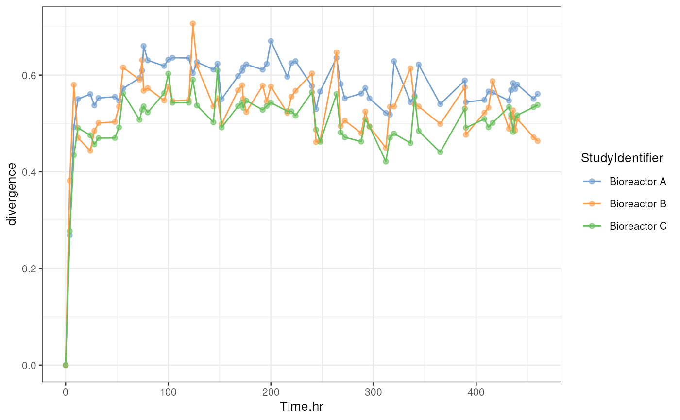

Visualizing selected taxa

Now visualize abundance of Blautia hydrogenotrophica using the miaViz::plotSeries() function.

library(miaViz)

# Plot certain feature by time
p <- plotSeries(
    tse,
    x = "Time.hr", y = "Blautia_hydrogenotrophica", colour_by = "Species",
    assay.type = "relabundance")
p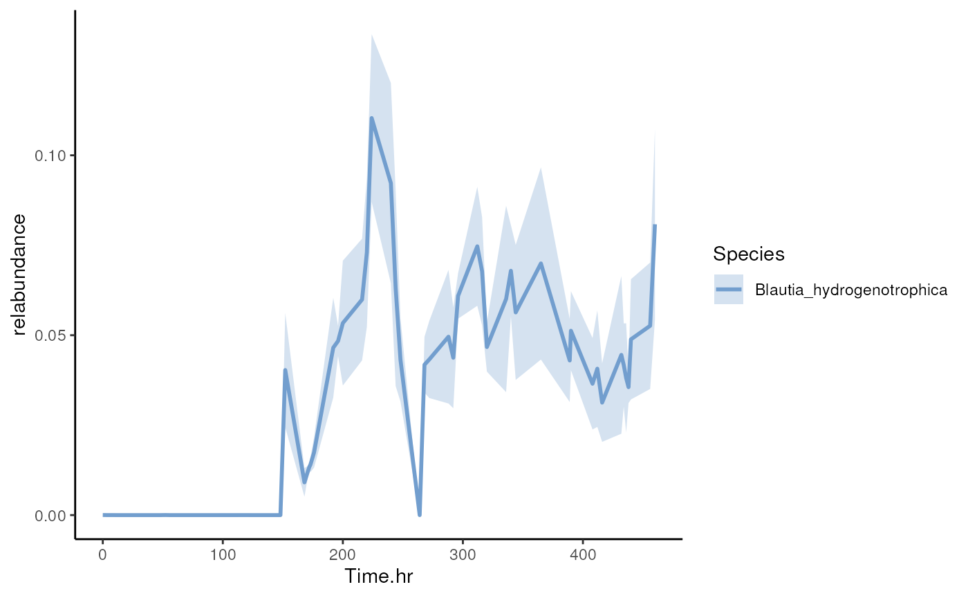

Visualize the rate (slope) of divergence

Sample dissimilarity between consecutive time steps(step size n >= 1) within a group(subject, age, reaction chamber, etc.) can be calculated by addStepwiseDivergence.

# Divergence between consecutive time points
tse <- addStepwiseDivergence(
    tse,
    assay.type = "relabundance",
    method = "bray",
    group = "StudyIdentifier",
    time.interval = 1,
    time.col = "Time.hr",
    name = c("divergence_from_previous_step", 
        "time_from_previous_step", "reference_samples")
    )

The results are again stored in colData. We calculate the speed of divergence change by dividing each divergence change by the corresponding change in time. Then we use similar plotting methods as previously.

# Calculate slope for the change
tse[["divergence_change"]] <- tse[["divergence_from_previous_step"]] /
    tse[["time_from_previous_step"]]

# Create a time series plot for divergence
p <- plotColData(
    tse,
    x = "Time.hr",
    y = "divergence_change",
    colour_by = "StudyIdentifier"
    ) +
    # Add line between points
    geom_line(aes(group = .data[["colour_by"]], colour =  .data[["colour_by"]]))
p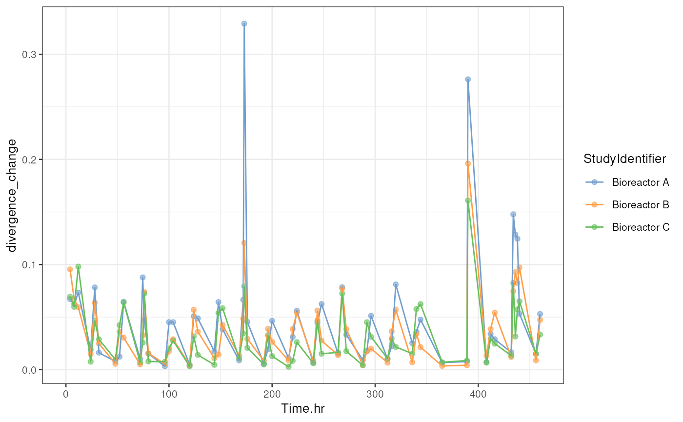

Moving average of the slope

This shows how to calculate and plot moving average for the variable of interest (here: slope).

library(dplyr)

# Calculate moving average with time window of 3 time points
tse[["sliding_divergence"]] <- colData(tse) |>
    as.data.frame() |>
    # Group based on reactor
    group_by(StudyIdentifier) |>
    # Calculate moving average
    mutate(sliding_avg = (
        # We get the previous 2 samples
        lag(divergence_change, 2) +
        lag(divergence_change, 1) +
        # And the current sample
        divergence_change
        # And take average
        ) / 3
    ) |>
    # Get only the values as vector
    ungroup() |>
    pull(sliding_avg)

After calculating the moving average of divergences, we can visualize the result in a similar way to our previous approach.

# Create a time series plot for divergence
p <- plotColData(
    tse,
    x = "Time.hr",
    y = "sliding_divergence",
    colour_by = "StudyIdentifier"
    ) +
    # Add line between points
    geom_line(aes(group = .data[["colour_by"]], colour =  .data[["colour_by"]]))
p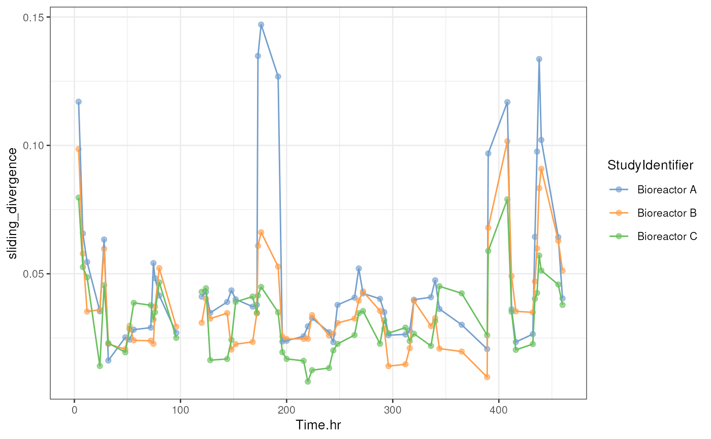

Session info