Alpha diversity

Estimated time: 105 minutes

Overview

Questions

• What is alpha diversity?
• How do we calculate alpha diversity?
• Does alpha diversity differ between people with colorectal cancer and healthy people?

Objectives

• Explain the difference between richness, evenness and diversity.
• Calculate alpha diversity indices with addAlpha().
• Plot alpha diversity by study group.
• Test whether alpha diversity differs between two groups with the Wilcoxon test, and interpret the result.

Where are we?

---

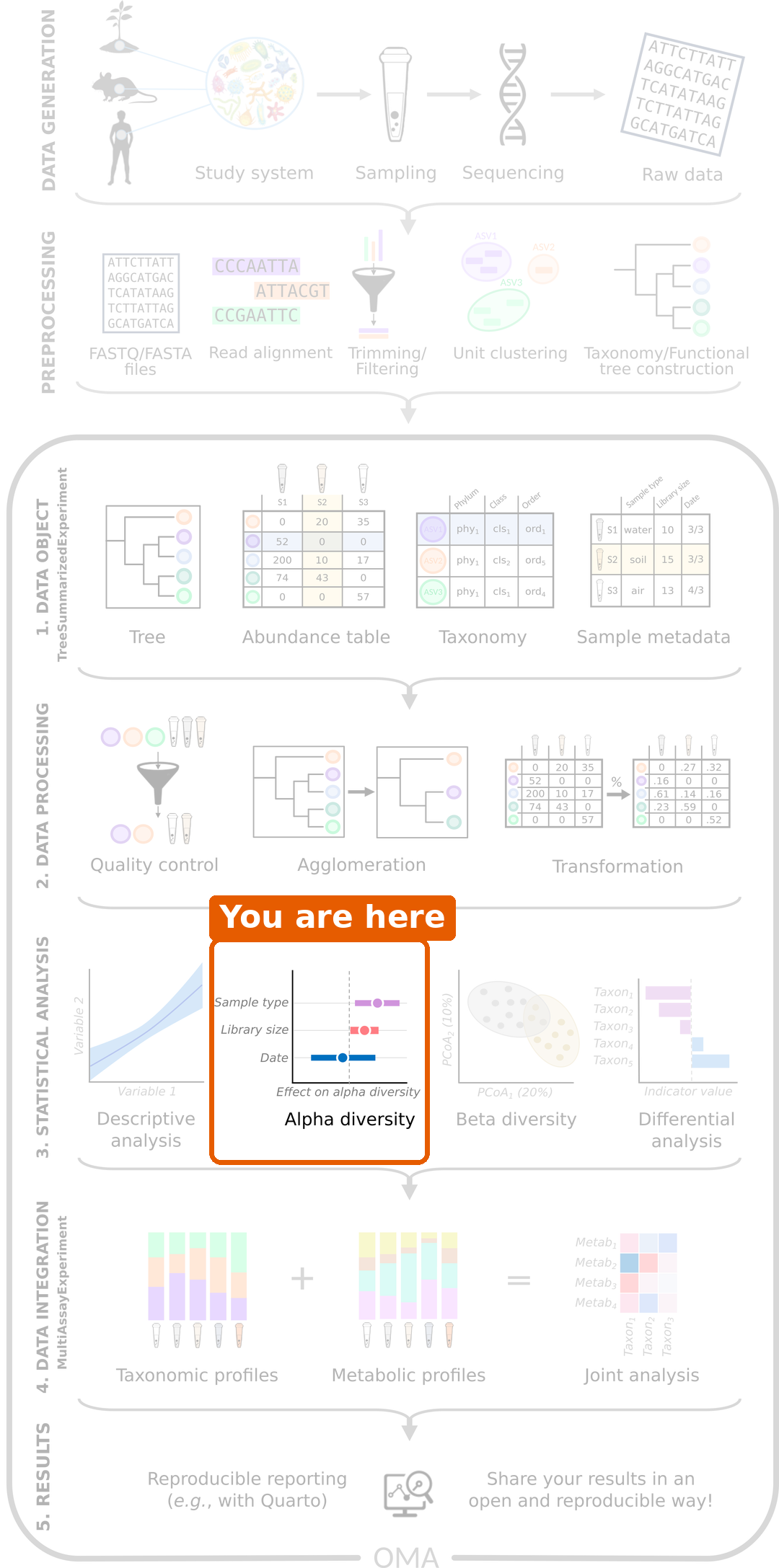
Our data is imported and processed. Now we start the statistical analysis that answers our research question. The first question is: do people with CRC and healthy people differ in the diversity of their gut microbiome?

Load packages and data

---

R

library(mia)
library(miaViz)

R

tse <- readRDS(file.path("data", "tse_processed.rds"))

What is alpha diversity?

---

Alpha diversity describes the diversity within one sample. Imagine two gardens with the same ten kinds of flowers:

• In garden A, all ten kinds are equally common.
• In garden B, one kind makes up 91 % of all flowers, and the other nine are rare.

In the picture below, each point is one flower and each colour is one kind:

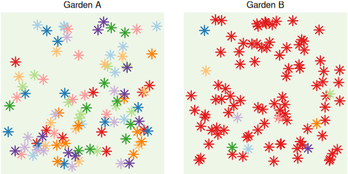
Both gardens have the same number of flower kinds, but garden A feels more diverse. Alpha diversity captures this with different measures, called indices:

Index	Question it answers	Values
Richness (observed richness)	How many different taxa are there?	The number of taxa
Evenness (Pielou’s evenness)	Are the taxa equally common, or do a few dominate?	From 0 (one taxon dominates) to 1 (all equally common)
Diversity (Shannon index)	Combines richness and evenness into one number.	From 0 upwards; typically 1–5 in gut samples
Phylogenetic diversity (Faith’s index)	How much of the tree of life do the taxa cover?	The total branch length of the tree

For all indices, a higher value means a more diverse sample.

These indices give complementary information. Two samples can have the same richness but a different evenness, as in the gardens above, or the same Shannon diversity for different reasons. Phylogenetic diversity adds whether the taxa are close relatives or come from distant branches of the tree. It is therefore good practice to look at several indices, not only one.

Challenge

Challenge 1: What does alpha diversity measure?

1. The diversity between different habitats
   
2. The diversity within a single community or habitat
   
3. The total number of ecosystems in a region

Show me the solution

2. The diversity within a single community or habitat. The differences between communities are called beta diversity, the topic of the next episode.

Challenge

Challenge 2: Two gardens

Look at gardens A and B in the figure above.

1. Which garden has the higher richness?
2. Which garden has the higher evenness?
3. Which garden has the higher Shannon diversity?

Show me the solution

1. Neither: both have ten kinds of flowers, so the richness is the same.
2. Garden A, because all kinds are equally common.
3. Garden A. Shannon diversity combines richness and evenness, and garden A has the same richness but a higher evenness.

Calculate alpha diversity

---

The function addAlpha() calculates alpha diversity indices from the counts. The transformations of the previous episode are not needed here. We choose the indices with the index argument:

R

tse <- addAlpha(
    tse, assay.type = "counts",
    index = c(
        "observed_richness", "pielou_evenness",
        "shannon_diversity", "faith_diversity"
    )
)

The results are added as new columns to colData, next to the other sample information:

R

colData(tse)[, c(
    "disease", "observed_richness", "pielou_evenness",
    "shannon_diversity", "faith_diversity"
)]

OUTPUT

DataFrame with 60 rows and 5 columns
               disease observed_richness pielou_evenness shannon_diversity
           <character>         <numeric>       <numeric>         <numeric>
GupDM_A_11         CRC                55        0.687513           2.75509
GupDM_A_15         CRC                29        0.310196           1.04452
GupDM_A1           CRC               149        0.665661           3.33093
GupDM_A10          CRC                69        0.653870           2.76856
GupDM_A12          CRC                64        0.633120           2.63307
...                ...               ...             ...               ...
GupDM_JL           CRC                46        0.684066           2.61904
GupDM_JM           CRC                70        0.682164           2.89817
GupDM_JN           CRC                71        0.685038           2.92010
GupDM_JO           CRC                89        0.696916           3.12820
GupDM_JP           CRC                86        0.778372           3.46714
           faith_diversity
                 <numeric>
GupDM_A_11         8.49226
GupDM_A_15         5.49297
GupDM_A1          17.55391
GupDM_A10          9.41595
GupDM_A12          9.41699
...                    ...
GupDM_JL           8.90981
GupDM_JM          11.20033
GupDM_JN          11.08878
GupDM_JO          13.03100
GupDM_JP          13.87034

Faith’s index needs the phylogenetic tree, which addAlpha() finds in the rowTree of the TreeSE.

Plot alpha diversity

---

The miaViz function plotBoxplot() shows the values of a colData column (col.var) for each group (x):

R

plotBoxplot(tse, col.var = "shannon_diversity", x = "disease")

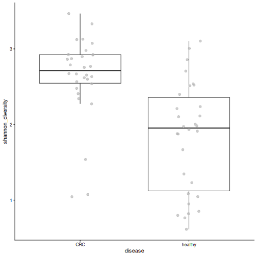
Each point is one person. The Shannon diversity appears higher in the CRC group. But is the difference larger than we would expect by chance?

Compare the groups with a statistical test

---

To compare two groups, we use the Wilcoxon test (also called the Mann–Whitney test). It sorts all values from smallest to largest and checks whether the values of one group tend to rank higher than those of the other. Because it uses only the order of the values, it does not assume that they follow a normal distribution, and a few extreme values do not distort it. This makes it a safe choice for diversity indices, which are often skewed. For more than two groups, the Kruskal–Wallis test (kruskal.test()) works in the same way.

The test gives a p-value: the probability of seeing a difference at least this large if the two groups did not really differ. In this lesson, we call a result significant when p < 0.05.

We run the test with daa::getWilcoxonTest() from the daa package. As explained in the setup episode, we write daa:: in front of its functions instead of loading the package. The formula reads “Shannon diversity by disease group”. The left side can be a column of colData, as here, or an assay, as we will see in the differential abundance episode.

R

shannon_test <- daa::getWilcoxonTest(tse, shannon_diversity ~ disease)
shannon_test

OUTPUT

# A tibble: 1 × 8
  rownames          .y.              group1 group2    n1    n2 statistic       p
* <chr>             <chr>            <chr>  <chr>  <int> <int>     <dbl>   <dbl>
1 shannon_diversity shannon_diversi… CRC    healt…    30    30       747 4.11e-6

Result: the median Shannon diversity is 2.71 in people with CRC and 1.95 in healthy people. The p-value is 4.1e-06, so the difference is very unlikely to be due to chance. People with CRC have a higher Shannon diversity than healthy people.

Challenge

Challenge 3: Richness

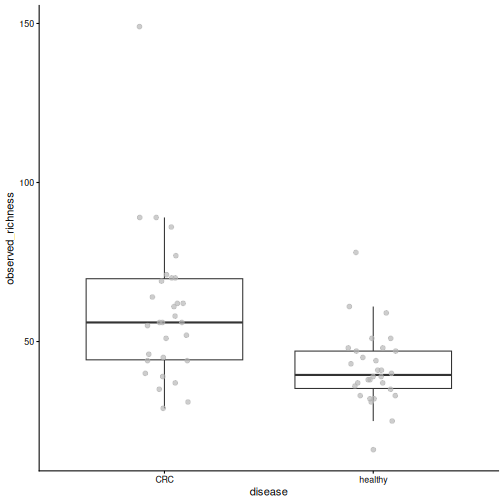
1. Plot the observed richness by disease group.
2. Test whether the richness differs between the groups.
3. Which group has more species?

Show me the solution

R

plotBoxplot(tse, col.var = "observed_richness", x = "disease")

R

richness_test <- daa::getWilcoxonTest(tse, observed_richness ~ disease)
richness_test

OUTPUT

# A tibble: 1 × 8
  rownames          .y.              group1 group2    n1    n2 statistic       p
* <chr>             <chr>            <chr>  <chr>  <int> <int>     <dbl>   <dbl>
1 observed_richness observed_richne… CRC    healt…    30    30      700. 1.35e-4

People with CRC have more species in their gut sample than healthy people (p = 0.00014).

Is higher diversity healthier?

---

A more diverse gut microbiome is often described as a healthy one. Why, then, is diversity lower in the healthy people of our study? Evenness gives a clue.

Challenge

Challenge 4: Evenness

1. Plot Pielou’s evenness by disease group. Which group is less even?
2. Think back to the previous episode: which species makes up about half of the community in many healthy people?
3. Use your answers to explain why healthy people have a lower Shannon diversity.

Show me the solution

R

plotBoxplot(tse, col.var = "pielou_evenness", x = "disease")

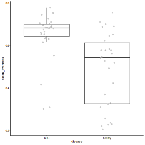
1. Healthy samples are less even.
2. Prevotella copri.
3. When one species takes up a large part of the community, the community is uneven, like garden B. A low evenness gives a low Shannon diversity.

So “higher diversity” does not automatically mean “healthier”. Diet, geography and lifestyle shape the gut microbiome, and Prevotella-dominated guts are common in many non-Western populations. Always interpret diversity in the context of the study.

Result: the median evenness is 0.54 in healthy people and 0.68 in people with CRC (p = 5.4e-05). The lower Shannon diversity of healthy people is largely due to their lower evenness: in many of them, one species dominates. Richness is higher in CRC too, so evenness is not the whole story. We will see in the next episodes which taxa differ between the groups.

Challenge

Challenge 5: Phylogenetic diversity

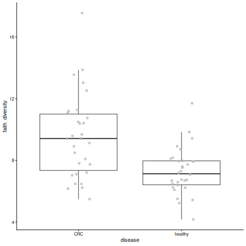
1. Does Faith’s phylogenetic diversity differ between the groups? Plot it and run the test.
2. Which part of the TreeSE does this index use that the other indices do not?

Show me the solution

R

plotBoxplot(tse, col.var = "faith_diversity", x = "disease")

R

faith_test <- daa::getWilcoxonTest(tse, faith_diversity ~ disease)
faith_test

OUTPUT

# A tibble: 1 × 8
  rownames        .y.             group1 group2     n1    n2 statistic        p
* <chr>           <chr>           <chr>  <chr>   <int> <int>     <dbl>    <dbl>
1 faith_diversity faith_diversity CRC    healthy    30    30       679 0.000543

1. Yes, it is higher in CRC (p = 0.00054).
2. The phylogenetic tree (rowTree). Faith’s index measures the total branch length of the tree covered by the taxa in a sample.

Callout

Sequencing depth and rarefaction

The deeper a sample is sequenced, the more rare taxa we find, so richness partly depends on the library size. This is often checked with rarefaction curves, or by randomly subsampling all samples to the same number of reads (rarefying). This applies to both amplicon and shotgun data; addAlpha() can rarefy with its sample and niter arguments.

Rarefying throws data away, and whether to do it is debated. A simple first check is whether richness is related to the library size. In our data, it is not clearly related (Spearman correlation rho = 0.16, p = 0.23), and the library sizes do not differ between the groups (p = 0.87), so we do not rarefy here. See the Alpha diversity chapter of OMA.

Challenge

Challenge 6: Diversity, age and gender (30 minutes)

Disease is not the only thing we know about the people in our study. Is diversity also related to their age or gender?

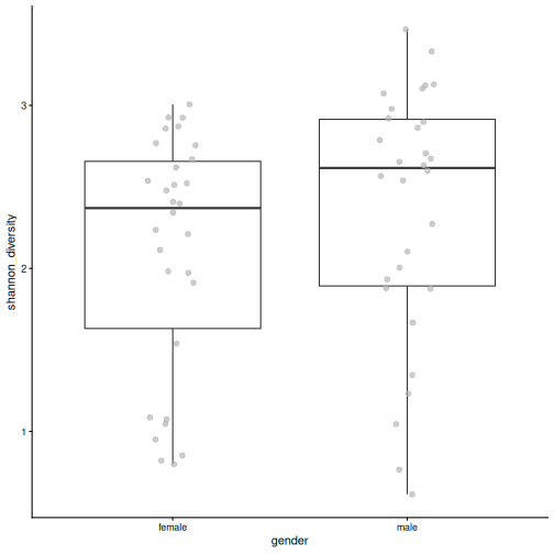
1. Does the Shannon diversity differ between women and men? Make the plot and run the test.
2. Is the Shannon diversity related to age? Use a correlation test: cor.test(tse$age, tse$shannon_diversity, method = "spearman").
3. Plot the age of the people by disease group. What do you notice?
4. Repeat the correlation test separately for the CRC patients and for the healthy people. Is diversity still related to age? Hint: subset the TreeSE to one group, as for any SummarizedExperiment: tse[, tse$disease == "CRC"].
5. Make age groups with tse$age_group <- cut(tse$age, breaks = c(0, 40, 60, 100), labels = c("under 40", "40-60", "over 60")) and plot the Shannon diversity by age group, coloured by disease (fill.by = "disease").
6. Write two or three sentences: is diversity related to age in this study?

Show me the solution

1. Gender

R

plotBoxplot(tse, col.var = "shannon_diversity", x = "gender")

R

gender_test <- daa::getWilcoxonTest(tse, shannon_diversity ~ gender)
gender_test

OUTPUT

# A tibble: 1 × 8
  rownames          .y.               group1 group2    n1    n2 statistic     p
* <chr>             <chr>             <chr>  <chr>  <int> <int>     <dbl> <dbl>
1 shannon_diversity shannon_diversity female male      30    30       346 0.127

There is no clear difference between women and men (p = 0.13).

2. Age

R

age_test <- cor.test(
    tse$age, tse$shannon_diversity, method = "spearman", exact = FALSE
)
age_test

OUTPUT

	Spearman's rank correlation rho

data:  tse$age and tse$shannon_diversity
S = 24173, p-value = 0.01043
alternative hypothesis: true rho is not equal to 0
sample estimates:
     rho
0.328331 

Older people seem to have a higher diversity (rho = 0.33, p = 0.01).

3. Age by disease

R

plotBoxplot(tse, col.var = "age", x = "disease")

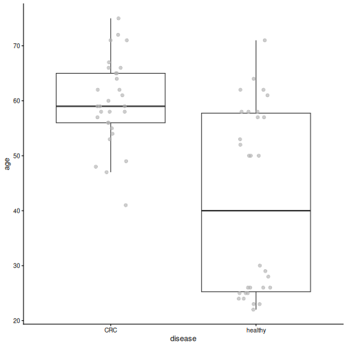
The CRC patients are much older (median 59 years) than the healthy people (median 40 years).

4. Within each group

R

tse_crc <- tse[, tse$disease == "CRC"]
age_test_crc <- cor.test(
    tse_crc$age, tse_crc$shannon_diversity, method = "spearman", exact = FALSE
)
age_test_crc

OUTPUT

	Spearman's rank correlation rho

data:  tse_crc$age and tse_crc$shannon_diversity
S = 3454.5, p-value = 0.2184
alternative hypothesis: true rho is not equal to 0
sample estimates:
      rho
0.2314807 

R

tse_healthy <- tse[, tse$disease == "healthy"]
age_test_healthy <- cor.test(
    tse_healthy$age, tse_healthy$shannon_diversity,
    method = "spearman", exact = FALSE
)
age_test_healthy

OUTPUT

	Spearman's rank correlation rho

data:  tse_healthy$age and tse_healthy$shannon_diversity
S = 4712.6, p-value = 0.7994
alternative hypothesis: true rho is not equal to 0
sample estimates:
        rho
-0.04841609 

Within each group, diversity is not clearly related to age (CRC: p = 0.22; healthy: p = 0.8).

5. Age groups

R

tse$age_group <- cut(
    tse$age, breaks = c(0, 40, 60, 100),
    labels = c("under 40", "40-60", "over 60")
)
plotBoxplot(
    tse, col.var = "shannon_diversity", x = "age_group", fill.by = "disease"
)

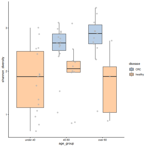
The youngest age group contains only healthy people. In the two older age groups, the CRC samples are more diverse than the healthy ones.

6. The link between age and diversity is most likely not a direct effect of age: it appears because the CRC patients, who have a higher diversity, are also older. Within each disease group, diversity is not clearly related to age, and within the same age group, CRC patients are still more diverse. When two variables are linked like this, it is called confounding (episode 1). We will meet it again with the location in episode 7. Always check how the variables in a study are related to each other.

Key Points

• Alpha diversity describes the diversity within a sample: richness (how many taxa), evenness (how equal), both (Shannon), or the share of the tree of life covered (Faith). The indices give complementary information.
• addAlpha() calculates diversity indices and adds them to colData.
• plotBoxplot() and daa::getWilcoxonTest() compare alpha diversity between two groups. The Wilcoxon test does not assume normally distributed values.
• In our study, people with CRC have a higher diversity, partly because the gut of many healthy people is dominated by one species. Higher diversity is not automatically healthier.
• Check for confounding: in our study, the CRC patients are also older than the healthy people.