Orchestrating Microbiome Analysis with Bioconductor
September-October 2026
Source:vignettes/example-workflow.Rmd
example-workflow.RmdAuthors: Tuomas Borman1, Leo Lahti
Last modified: 17
September, 2026.


Overview
Description
This training session introduces Bioconductor tools for microbiome and multiomics data science through a practical case study. It focuses on a framework built around TreeSummarizedExperiment and MultiAssayExperiment data containers, designed for improved efficiency, scalability, and integrated analysis of multiple omics layers. Participants will gain hands-on experience with common analysis and visualization methods using the mia package family and other multiomics-compatible tools from the Bioconductor ecosystem. After the session, participants can continue learning through the freely available Orchestrating Microbiome Analysis (OMA) online book.
Pre-requisites
To get most of the training session, you should meet the following pre-requisites.
- You have a basic understanding of R. You have written simple R scripts or used Quarto/RMarkdown documents.
- You are familiar with Bioconductor.
- You have basic understanding on what the microbiome is.
If your time allows, we recommend to spend some time to explore beforehand Orchestrating Microbiome Analysis (OMA) online book.
Training session
Import data
In this workshop, we analyze data from the study by (Gupta et al. 2019). The dataset contains samples from patients with colorectal cancer (CRC) and healthy individuals. In the study, metagenomic data were collected from stool samples, with the aim of identifying microbial factors that may contribute to the development of the disease.
The first step is to import the data. For standardized data formats,
such as those generated by MetaPhlAn and HUMAnN, Bioconductor provides
dedicated importers. However, a TreeSummarizedExperiment
(TreeSE) object can also be constructed manually, which is
what we will do in this workshop.
First, we need to load the data files into the R session.
library(ape)

dir_name <- "data"

# Abundance table
path <- file.path(dir_name, "taxonomy_abundance.csv")
assay <- read.csv(path, row.names = 1L)

# Taxonomy table
path <- file.path(dir_name, "taxonomy_table.csv")
taxonomy_table <- read.csv(path, row.names = 1L)

# Sample metadata
path <- file.path(dir_name, "sample_metadata.csv")
sample_metadata <- read.csv(path, row.names = 1L)

# Phylogeny
path <- file.path(dir_name, "phylogeny.tree")
phylogeny <- read.tree(path)
Then we create TreeSE object. Note:
data types must be in specific format.
library(mia)
# Abundance table
assay <- assay |> as.matrix()
assay_list <- SimpleList(counts = assay)

# Taxonomy table and sample metadata
taxonomy_table <- taxonomy_table |> DataFrame()
sample_metadata <- sample_metadata |> DataFrame()

# Construct TreeSE
tse <- TreeSummarizedExperiment(
    assays = assay_list,
    rowData = taxonomy_table,
    colData = sample_metadata,
    rowTree = phylogeny
)
tse
#> class: TreeSummarizedExperiment
#> dim: 308 60
#> metadata(0):
#> assays(1): counts
#> rownames(308): species-Escherichia_coli species-Alistipes_putredinis
#>   ... species-Campylobacter_ureolyticus
#>   species-Prevotella_sp._oral_taxon_376
#> rowData names(7): superkingdom phylum ... genus species
#> colnames(60): GupDM_A_11 GupDM_A_15 ... GupDM_JO GupDM_JP
#> colData names(27): study_name subject_id ... disease_stage
#>   disease_location
#> reducedDimNames(0):
#> mainExpName: NULL
#> altExpNames(0):
#> rowLinks: a LinkDataFrame (308 rows)
#> rowTree: 1 phylo tree(s) (10430 leaves)
#> colLinks: NULL
#> colTree: NULL
A TreeSE consists of slots that store different types of
data. For example, the colData slot stores sample-level
metadata, such as disease status, age, or sex.
Data can be accessed using functions named after the corresponding
slots. For example, colData() retrieves the sample metadata
from the TreeSE object.
colData(tse)
#> DataFrame with 60 rows and 27 columns
#>             study_name  subject_id   body_site antibiotics_current_use
#>            <character> <character> <character>             <character>
#> GupDM_A_11 GuptaA_2019   GupDM_A11       stool                      no
#> GupDM_A_15 GuptaA_2019   GupDM_A15       stool                      no
#> GupDM_A1   GuptaA_2019    GupDM_A1       stool                      no
#> GupDM_A10  GuptaA_2019   GupDM_A10       stool                      no
#> GupDM_A12  GuptaA_2019   GupDM_A12       stool                      no
#> ...                ...         ...         ...                     ...
#> GupDM_JL   GuptaA_2019    GupDM_JL       stool                      no
#> GupDM_JM   GuptaA_2019    GupDM_JM       stool                      no
#> GupDM_JN   GuptaA_2019    GupDM_JN       stool                      no
#> GupDM_JO   GuptaA_2019    GupDM_JO       stool                      no
#> GupDM_JP   GuptaA_2019    GupDM_JP       stool                      no
#>            study_condition     disease       age age_category      gender
#>                <character> <character> <integer>  <character> <character>
#> GupDM_A_11             CRC         CRC        41        adult      female
#> GupDM_A_15             CRC         CRC        59        adult        male
#> GupDM_A1               CRC         CRC        62        adult        male
#> GupDM_A10              CRC         CRC        65        adult      female
#> GupDM_A12              CRC         CRC        65        adult        male
#> ...                    ...         ...       ...          ...         ...
#> GupDM_JL               CRC         CRC        59        adult      female
#> GupDM_JM               CRC         CRC        60        adult        male
#> GupDM_JN               CRC         CRC        58        adult        male
#> GupDM_JO               CRC         CRC        71       senior        male
#> GupDM_JP               CRC         CRC        67       senior        male
#>                country    location non_westernized sequencing_platform
#>            <character> <character>     <character>         <character>
#> GupDM_A_11         IND      Kerala              no     IlluminaNextSeq
#> GupDM_A_15         IND      Kerala              no     IlluminaNextSeq
#> GupDM_A1           IND      Kerala              no     IlluminaNextSeq
#> GupDM_A10          IND      Kerala              no     IlluminaNextSeq
#> GupDM_A12          IND      Kerala              no     IlluminaNextSeq
#> ...                ...         ...             ...                 ...
#> GupDM_JL           IND      Bhopal              no     IlluminaNextSeq
#> GupDM_JM           IND      Bhopal              no     IlluminaNextSeq
#> GupDM_JN           IND      Bhopal              no     IlluminaNextSeq
#> GupDM_JO           IND      Bhopal              no     IlluminaNextSeq
#> GupDM_JP           IND      Bhopal              no     IlluminaNextSeq
#>            DNA_extraction_kit      PMID number_reads number_bases
#>                   <character> <integer>    <integer>    <numeric>
#> GupDM_A_11             Qiagen  31719139      6227234    883347281
#> GupDM_A_15             Qiagen  31719139      9884266   1384530792
#> GupDM_A1               Qiagen  31719139     27687226   3808647004
#> GupDM_A10              Qiagen  31719139      8468208   1174245166
#> GupDM_A12              Qiagen  31719139      6988838    984235167
#> ...                       ...       ...          ...          ...
#> GupDM_JL               Qiagen  31719139      9878044   1387793557
#> GupDM_JM               Qiagen  31719139     10328094   1435043694
#> GupDM_JN               Qiagen  31719139      9789278   1347588954
#> GupDM_JO               Qiagen  31719139     11274338   1501226163
#> GupDM_JP               Qiagen  31719139     10400668   1428270555
#>            minimum_read_length median_read_length NCBI_accession
#>                      <integer>          <integer>    <character>
#> GupDM_A_11                  60                151     SRR8865600
#> GupDM_A_15                  60                150     SRR8865596
#> GupDM_A1                    60                150     SRR8865598
#> GupDM_A10                   60                150     SRR8865599
#> GupDM_A12                   60                150     SRR8865601
#> ...                        ...                ...            ...
#> GupDM_JL                    60                151     SRR8865572
#> GupDM_JM                    60                150     SRR8865575
#> GupDM_JN                    60                150     SRR8865574
#> GupDM_JO                    60                150     SRR8865581
#> GupDM_JP                    60                150     SRR8865580
#>                           curator       BMI disease_subtype         tnm
#>                       <character> <numeric>     <character> <character>
#> GupDM_A_11 Arianna_Bonetti;Paol..     19.22  adenocarcinoma      t2m0n0
#> GupDM_A_15 Arianna_Bonetti;Paol..     21.40  adenocarcinoma      t2n0m0
#> GupDM_A1   Arianna_Bonetti;Paol..     20.08  adenocarcinoma      t2n0m0
#> GupDM_A10  Arianna_Bonetti;Paol..     21.01  adenocarcinoma      t3n2m0
#> GupDM_A12  Arianna_Bonetti;Paol..     20.32  adenocarcinoma      t2n2m0
#> ...                           ...       ...             ...         ...
#> GupDM_JL   Arianna_Bonetti;Paol..     20.34  adenocarcinoma      t4n1m0
#> GupDM_JM   Arianna_Bonetti;Paol..     18.33  adenocarcinoma      t2n0m0
#> GupDM_JN   Arianna_Bonetti;Paol..     19.92  adenocarcinoma      t2n0m0
#> GupDM_JO   Arianna_Bonetti;Paol..     20.03  adenocarcinoma      t4n1m0
#> GupDM_JP   Arianna_Bonetti;Paol..     17.69  adenocarcinoma      t3n2m0
#>                   fobt disease_stage disease_location
#>            <character>   <character>      <character>
#> GupDM_A_11         yes             I           rectum
#> GupDM_A_15         yes             I           rectum
#> GupDM_A1           yes             I           rectum
#> GupDM_A10          yes           III            colon
#> GupDM_A12          yes           III           rectum
#> ...                ...           ...              ...
#> GupDM_JL           yes           III           rectum
#> GupDM_JM           yes             I           rectum
#> GupDM_JN           yes             I           rectum
#> GupDM_JO           yes           III    sigmoid_colon
#> GupDM_JP           yes           III           rectum
A TreeSE object contains rows and columns and can be
subsetted similarly to other rectangular objects in R. Below, we select
the first row (i.e., one bacterial feature) and samples 10–13.
tse[1, 10:13]
#> class: TreeSummarizedExperiment
#> dim: 1 4
#> metadata(0):
#> assays(1): counts
#> rownames(1): species-Escherichia_coli
#> rowData names(7): superkingdom phylum ... genus species
#> colnames(4): GupDM_A4 GupDM_A5 GupDM_A6 GupDM_A7
#> colData names(27): study_name subject_id ... disease_stage
#>   disease_location
#> reducedDimNames(0):
#> mainExpName: NULL
#> altExpNames(0):
#> rowLinks: a LinkDataFrame (1 rows)
#> rowTree: 1 phylo tree(s) (10430 leaves)
#> colLinks: NULL
#> colTree: NULL
Agglomeration
Agglomeration is commonly used to reduce the number of features or to focus on biologically meaningful subgroups of the data. Agglomeration means merging data into higher taxonomic levels by summing the abundances of related taxa.
Below, we agglomerate the data into all available taxonomy levels.
library(mia)

tse <- agglomerateByRanks(tse)
At first glance, it might seem that nothing has changed. However, the
agglomerated data is stored in the altExp slot. This slot
keeps track of the sample mapping and stores different versions of the
data.
We can access data agglomeration into the phylum level with the following command:
altExp(tse, "phylum")
#> class: TreeSummarizedExperiment
#> dim: 11 60
#> metadata(1): agglomerated_by_rank
#> assays(1): counts
#> rownames(11): Actinobacteria Bacteroidota ... Synergistetes
#>   Verrucomicrobia
#> rowData names(7): superkingdom phylum ... genus species
#> colnames(60): GupDM_A_11 GupDM_A_15 ... GupDM_JO GupDM_JP
#> colData names(27): study_name subject_id ... disease_stage
#>   disease_location
#> reducedDimNames(0):
#> mainExpName: NULL
#> altExpNames(0):
#> rowLinks: a LinkDataFrame (11 rows)
#> rowTree: 1 phylo tree(s) (11 leaves)
#> colLinks: NULL
#> colTree: NULL
The data looks similar to original data; only the number of rows has
changed. While we could store the phylum-level data in a separate
variable, it’s better to keep it in the altExp slot, as it
maintains consistent sample mapping for us.
Transformation
Another data processing step where microbiome analysis has unique approaches is transformation. Microbiome data is typically zero-inflated:
library(miaViz)

plotHistogram(tse, assay.type = "counts")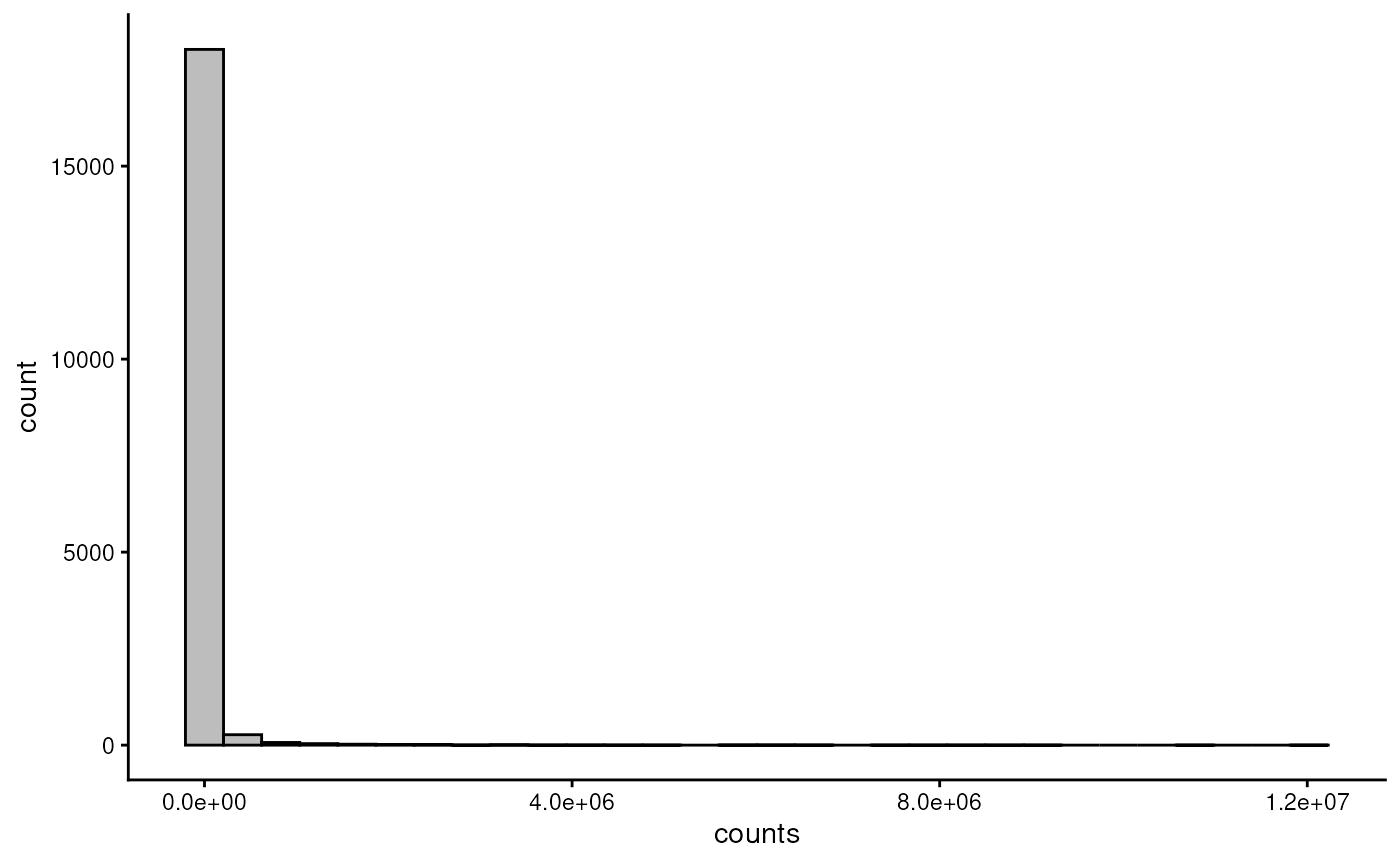
Below, we apply centered log-ratio (CLR) transformations which respect the compositional nature of microbiome data.
tse <- transformAssay(
    tse,
    assay.type = "counts",
    method = "rclr",
    altexp = altExpNames(tse)
)
By visualixing the CLR-transofrmed data, we see that the data is now centered to zero without constrains; suitable for classical statistical tests.
plotHistogram(tse, assay.type = "rclr")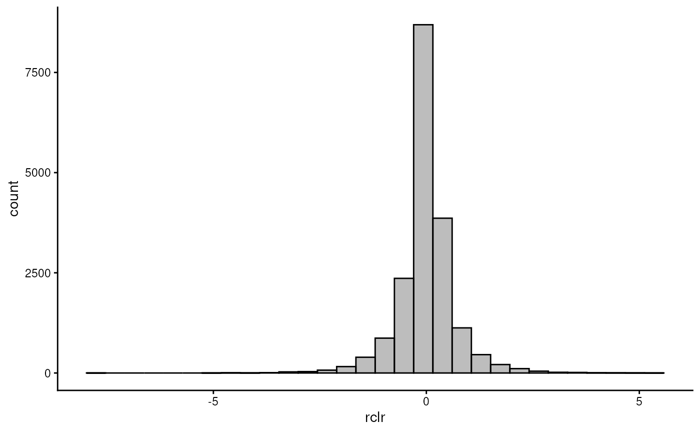
Another common transformation is relative transformation.
tse <- transformAssay(
    tse,
    assay.type = "counts",
    method = "relabundance",
    altexp = altExpNames(tse)
)
We can see that the transformed table is added to the same data
object. We can access the table with assay() command.
assay(tse, "relabundance")[1:2, 1:3]
#>                              GupDM_A_11 GupDM_A_15    GupDM_A1
#> species-Escherichia_coli      0.2621285  0.5733251 0.246128460
#> species-Alistipes_putredinis  0.1549458  0.0000000 0.008134657
Community composition
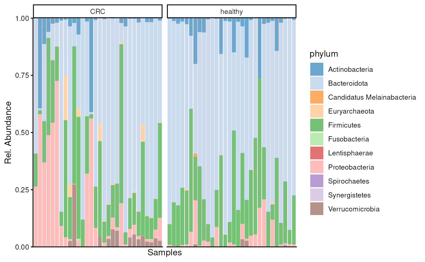
While mia package include common methods for analysis, miaViz provides methods for visualizing microbiome data. For instance, we can visualize abundance of phyla with a bar plot. To compare study groups, we can visualize them separately.
# Create a bar plot
plotAbundance(
    tse,
    assay.type = "counts",
    as.relative = TRUE,
    rank = "phylum",
    col.var = "disease"
)
Alpha diversity
To summarize the diversity of microbial communities, alpha diversity is commonly calculated. There are several diversity indices available, all of which measure the number of distinct taxa and how evenly their abundances are distributed, each with a different emphasis.
tse <- addAlpha(tse, assay.type = "counts")The results are stored in colData. By default,
addAlpha() returns a set of indices that considers
different aspects of diversity. Commonly, the results are visualized
with a box plot.
Below, we visualize Faith’s phylogenetic diversity, an alpha-diversity measure that incorporates information from the phylogenetic tree.
The advantage of using a phylogenetic diversity measure is that it accounts for the evolutionary relationships between microbial features. Not all bacteria are equally related: some taxa are more closely related than others. Incorporating this information allows us to distinguish between communities that may have the same number of taxa but differ in their phylogenetic breadth, preserving information that would be lost with non-phylogenetic diversity measures.
plotBoxplot(tse, col.var = "faith_diversity", x = "disease")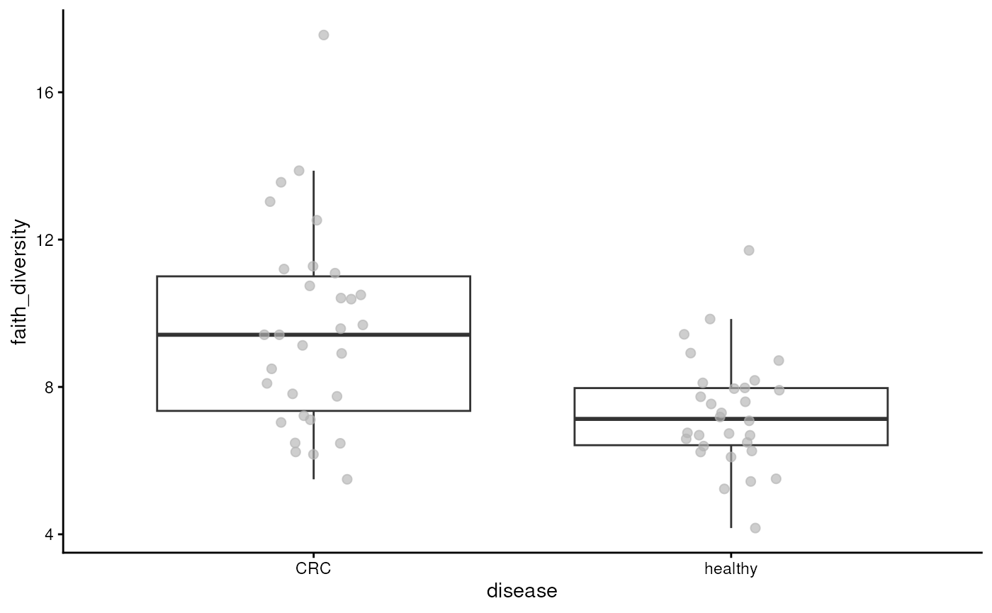
To test the statistical significance of results, we can do Wilcoxon test.
library(daa)

getWilcoxonTest(tse, formula = faith_diversity ~ disease)
#> # A tibble: 1 × 8
#>   rownames        .y.             group1 group2     n1    n2 statistic        p
#> * <chr>           <chr>           <chr>  <chr>   <int> <int>     <dbl>    <dbl>
#> 1 faith_diversity faith_diversity CRC    healthy    30    30       679 0.000543
Beta diversity
While alpha diversity reflects within-sample diversity, beta diversity measures diversity between samples. This allows us to assess whether there are patterns in microbial profiles associated with covariates.
Below, we apply Principal Coordinate Analysis (PCoA), also known as multidimensional scaling (MDS). PCoA is similar to Principal Component Analysis (PCA), but instead of operating directly on the original feature matrix, it starts with a dissimilarity or distance matrix.
Several distance measures can be used with PCoA. One of them is UniFrac, which incorporates the phylogenetic relationships between microbial taxa when calculating differences between microbial communities. This allows PCoA based on UniFrac distances to capture differences in both community composition and evolutionary relatedness.
tse <- addMDS(
    tse,
    assay.type = "counts",
    method = "unifrac"
)
The data is stoed to reducedDim slot of
TreeSE. Common way to visualize the results is to create a
scatter plot.
plotOrdination(tse, dimred = "MDS", colour.by = "disease")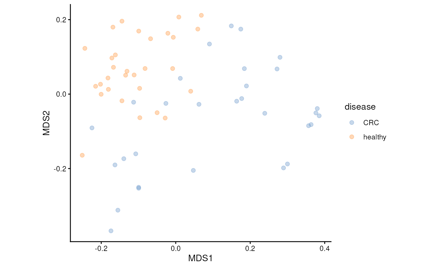
Differential abundance/prevalence analysis
In differential abundance analysis (DAA), we examine each bacterial feature individually and test whether its abundance differs between study groups. For example, we can ask whether Bacterium X is more abundant in CRC patients than in healthy individuals.
Recent studies suggest that differential prevalence analysis (DPA) can provide a more robust alternative in some settings. Instead of comparing abundance, DPA asks whether a microbial feature is detected more frequently in one group than another.
MaAsLin3 (Nickols et al. 2024) supports both differential abundance and differential prevalence analyses.
library(maaslin3)

# Helper for catching all printing from Maaslin3 and IL
quiet <- function(x) {
    invisible(capture.output(x))
    return(x)
}

res <- maaslin3(tse, formula = ~ disease, output = "maaslin3_output") |> quiet()
Maalsin3 generates summary figure.
file_path <- file.path("maaslin3_output", "figures", "summary_plot.png")
knitr::include_graphics(file_path)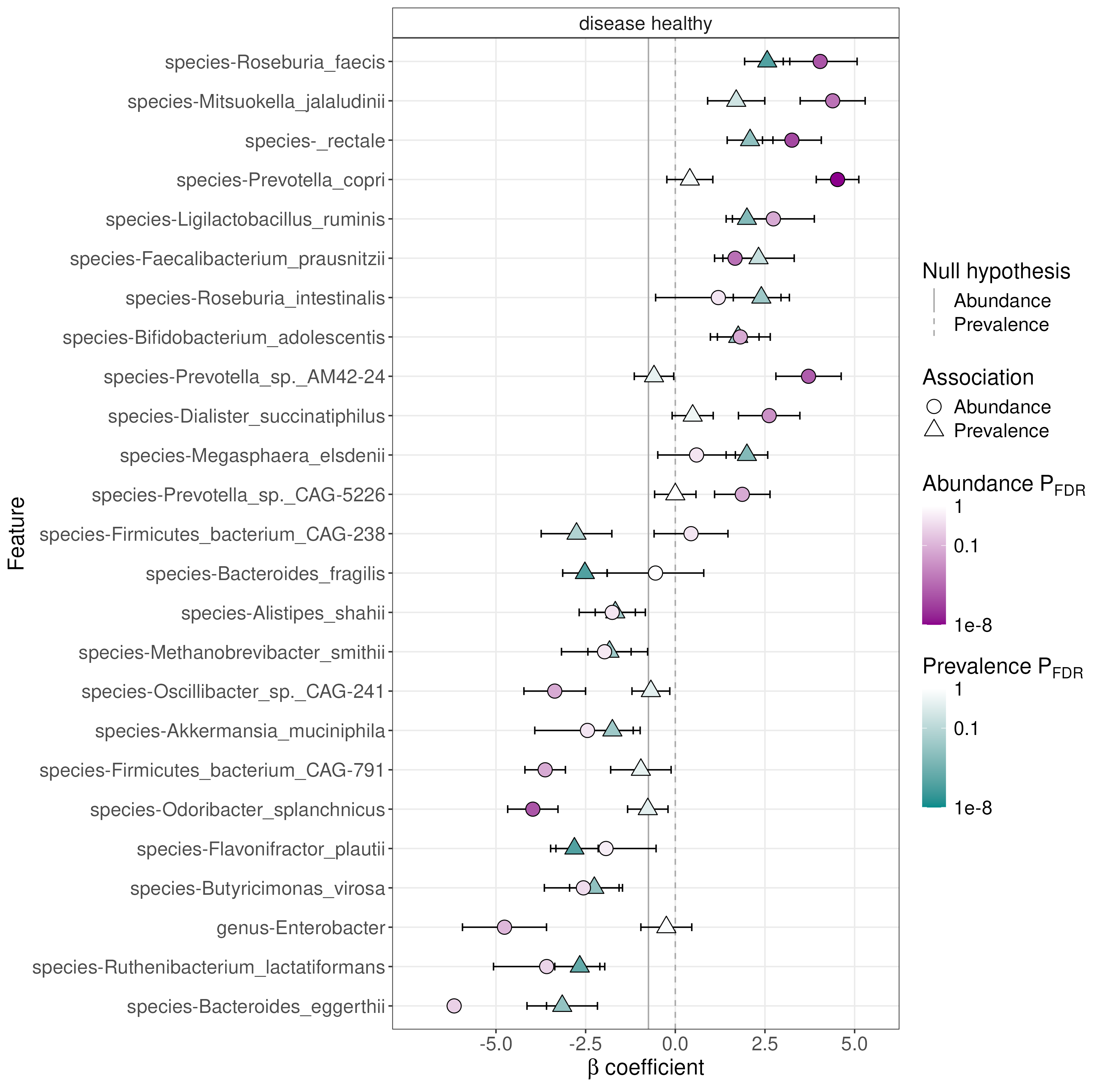
Import additional omic layer
The dataset contains functional pathway information in addition to
taxonomic profiles. We import the pathway data in the same way as the
taxonomy data and store it in a TreeSE data container. Then
we wrap these two omics into MAE data container.
Let’s first import pathways into TreeSE.
dir_name <- "data"

# Abundance table
path <- file.path(dir_name, "pathway_abundance.csv")
assay <- read.csv(path, row.names = 1L)

# Abundance table
assay <- assay |> as.matrix()
assay_list <- SimpleList(relative_abundance = assay)

# Sample metadata
sample_metadata <- sample_metadata |> DataFrame()

# Construct TreeSE
tse2 <- TreeSummarizedExperiment(
    assays = assay_list,
    colData = sample_metadata
)
Now when we have also pathways in TreeSE format, we can
wrap them with MAE. It can be seen as a list of
TreeSE objects with additional sampleMap
functionality that links samples between omic layers.
mae <- MultiAssayExperiment(
    experiments = ExperimentList(
        taxonomy = tse,
        pathway = tse2
    ),
    colData = sample_metadata
)
mae
#> A MultiAssayExperiment object of 2 listed
#>  experiments with user-defined names and respective classes.
#>  Containing an ExperimentList class object of length 2:
#>  [1] taxonomy: TreeSummarizedExperiment with 308 rows and 60 columns
#>  [2] pathway: TreeSummarizedExperiment with 50 rows and 60 columns
#> Functionality:
#>  experiments() - obtain the ExperimentList instance
#>  colData() - the primary/phenotype DataFrame
#>  sampleMap() - the sample coordination DataFrame
#>  `$`, `[`, `[[` - extract colData columns, subset, or experiment
#>  *Format() - convert into a long or wide DataFrame
#>  assays() - convert ExperimentList to a SimpleList of matrices
#>  exportClass() - save data to flat files
In this dataset, the same samples are measured across both omics
layers. However, the sampleMap structure allows flexible
mapping between samples across experiments, so the omics layers do not
need to contain exactly the same set of samples. This is useful when
some samples are missing from one omics layer or when samples have
different identifiers across datasets.
Next we apply CLR-transformation to pathways. Note that the experiment or layer can be accessed similarly to list.
mae[[2]] <- transformAssay(
    mae[[2]],
    assay.type = "relative_abundance",
    method = "rclr",
    pseudocount = TRUE
)
Data integration
In recent years, many different approaches to integrate multiomics data has been proposed. For instance, (Mangnier et al. 2025) benchmarked different approaches to integrate metagenomics and metabolomics data, and evaluated different methods based on robustness and interpretability.
In the publication, they proposed the following methods to address the following research questions:
| Scientific question | Research aim | Recommended method |
|---|---|---|
| Is there any relationship between microorganisms and metabolites at a global level? | Global associations | Mantel test |
| Are microbiome and metabolome datasets summarizable through a limited number of components? | Data summarization | RDA |
| Can we identify associations between metabolites and species? | Individual associations | MiRKAT |
| Can we identify core microorganisms and metabolites? | Feature selection (univariate) | CODA-LASSO (compositional covariates) |
These methods are implemented in multiomics package that
supports MAE data container.
Mantel test
Usually it is wise to go from simpler methods to more complex.
The Mantel test calculates a dissimilarity matrix for each omics layer separately. It then compares the two matrices to determine whether the patterns of differences between samples are similar across the two layers.
If samples that are taxonomically similar in layer 1 are also similar in layer 2, and samples that are dissimilar in layer 1 are also dissimilar in layer 2, this indicates a global association between the two omics layers.
library(multiomics)

mantel <- getMantel(
    mae,
    experiments = c(1, 2),
    assay.types = c("rclr", "rclr"),
    dist.methods = c("euclidean", "euclidean")
)
mantel
#>
#> Mantel statistic based on Kendall's rank correlation tau
#>
#> Call:
#> mantel(xdis = x[[1L]], ydis = x[[2L]], method = method, permutations = npermutations,      strata = strata, na.rm = na.rm, parallel = parallel)
#>
#> Mantel statistic r: 0.154
#>       Significance: 0.001
#>
#> Upper quantiles of permutations (null model):
#>    90%    95%  97.5%    99%
#> 0.0520 0.0701 0.0845 0.0974
#> Permutation: free
#> Number of permutations: 999
Kendall’s tau correlation shows samples that are relatively similar in their taxonomic composition tend to be relatively similar in their pathway composition, but the relationship is weak.
MiRKAT
MiRKAT (Microbiome Regression-based Kernel Association Test) can be used to investigate whether specific microbial pathways are significantly associated with overall microbial community composition. Unlike the Mantel test, which evaluates the global association between two entire dissimilarity matrices, MiRKAT can help identify individual pathways whose variation across samples is associated with differences in the microbial profile.
mirkat <- getMiRKAT(
    mae,
    experiments = c(1, 2),
    assay.types = c("rclr", "rclr"),
    altexp = c("family", NA),
    dist.methods = "euclidean"
)
plot(mirkat)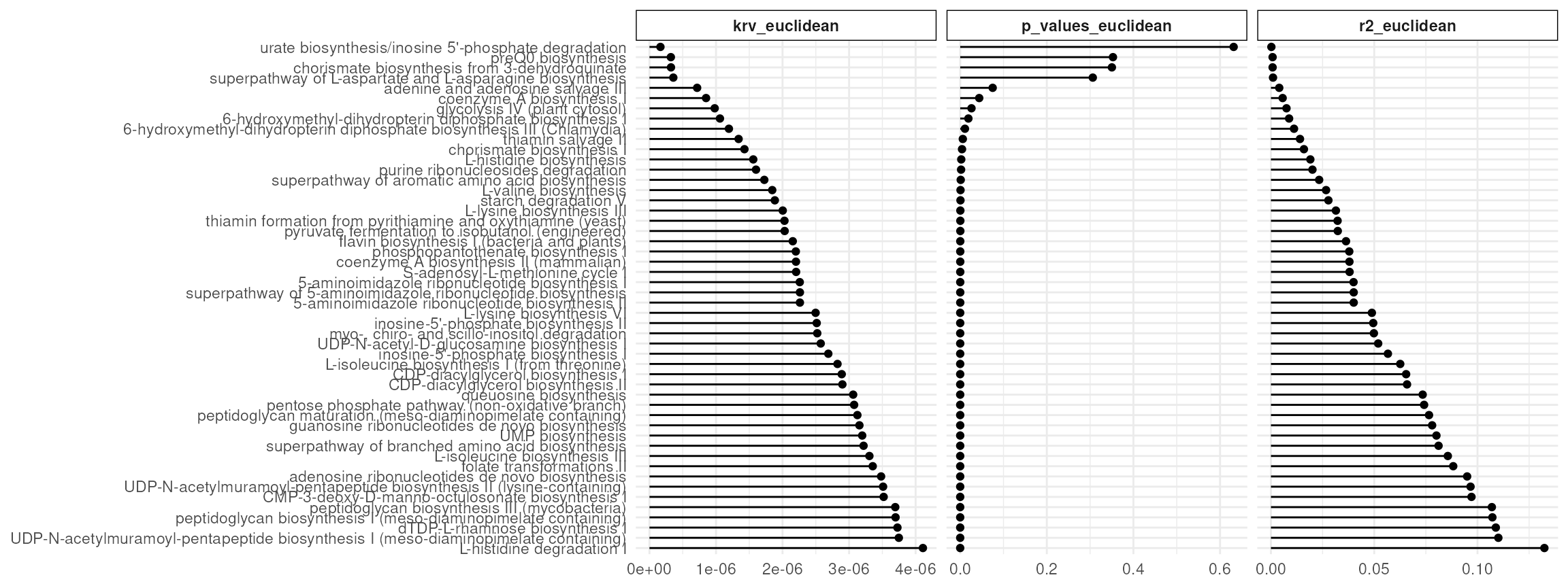
Pairwise association
Now that we know that the microbial profiles are associated with certain pathways, we can examine these relationships in more detail. One simple approach is to calculate pairwise associations between all taxon–pathway pairs and visualize the results as a heatmap. This allows us to identify specific taxa and pathways that show strong positive or negative associations.
cor <- getPairwiseAssociation(
    mae,
    experiments = c(1, 2),
    assay.types = c("rclr", "rclr"),
    altexp = c("phylum", NA)
)

plot(cor)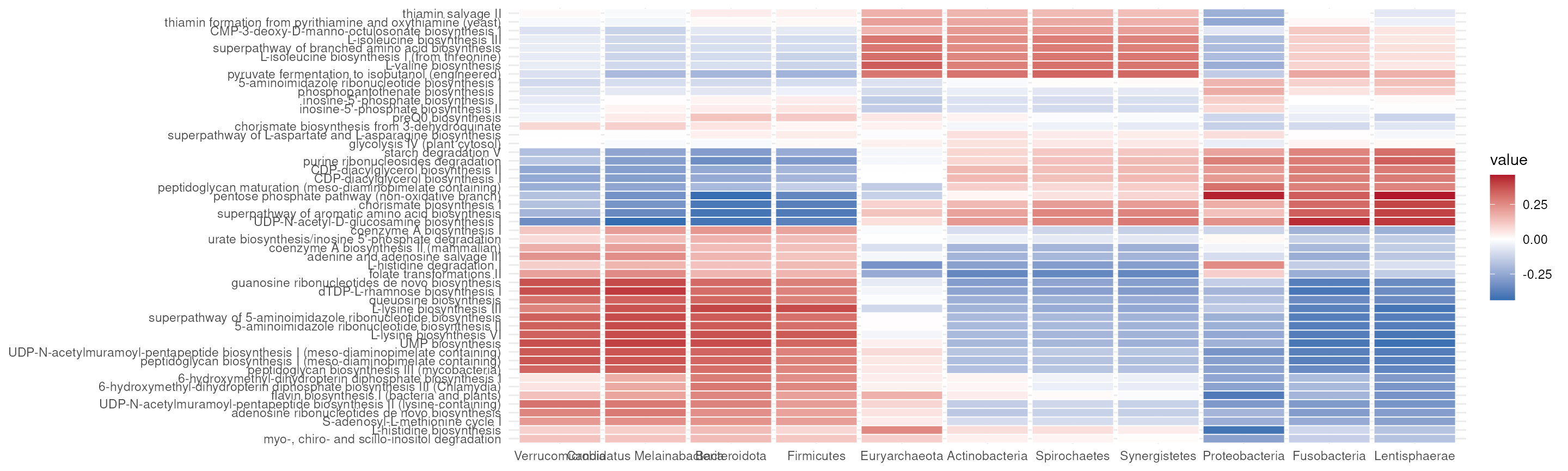
Joint robust principal component analysis
Although correlation-based approaches are simple and easy to interpret, they generally focus on pairwise relationships and may not adequately capture the complex, multivariate structure of microbial communities. Microbes interact as networks, so it can be useful to identify patterns of variation shared across multiple features and omics layers.
To account for this, we can use joint robust principal component analysis (joint RPCA) (Cordazzo Vargas et al. 2026). The method identifies a shared lower-dimensional representation of the samples across the omics layers, while allowing features from different layers to have different weights to account for differences in scale and variability. This reduces the influence of noise and features with very large values.
PCA is then applied to this integrated representation to identify the major axes of variation. The resulting principal components (latent factors) can be associated with clinical or other outcomes to determine whether the shared multi-omics variation is related to the outcome.
Finally, by examining the feature loadings of the components, we can identify which microbial taxa, pathways, or other features contribute most strongly to the shared patterns of variation across the omics layers.
# Run joint-RPCA
mae <- addJointRPCA(
   mae,
   experiments = c(1, 2),
   altexp = c("family", NA),
   assay.types = c("rclr", "rclr")
)
The result can be visualize with a scatter plot similarly to regular PCA.
library(miaViz)

plotJointRPCA(mae, "JointRPCA", ntop = 5, colour.by = "disease")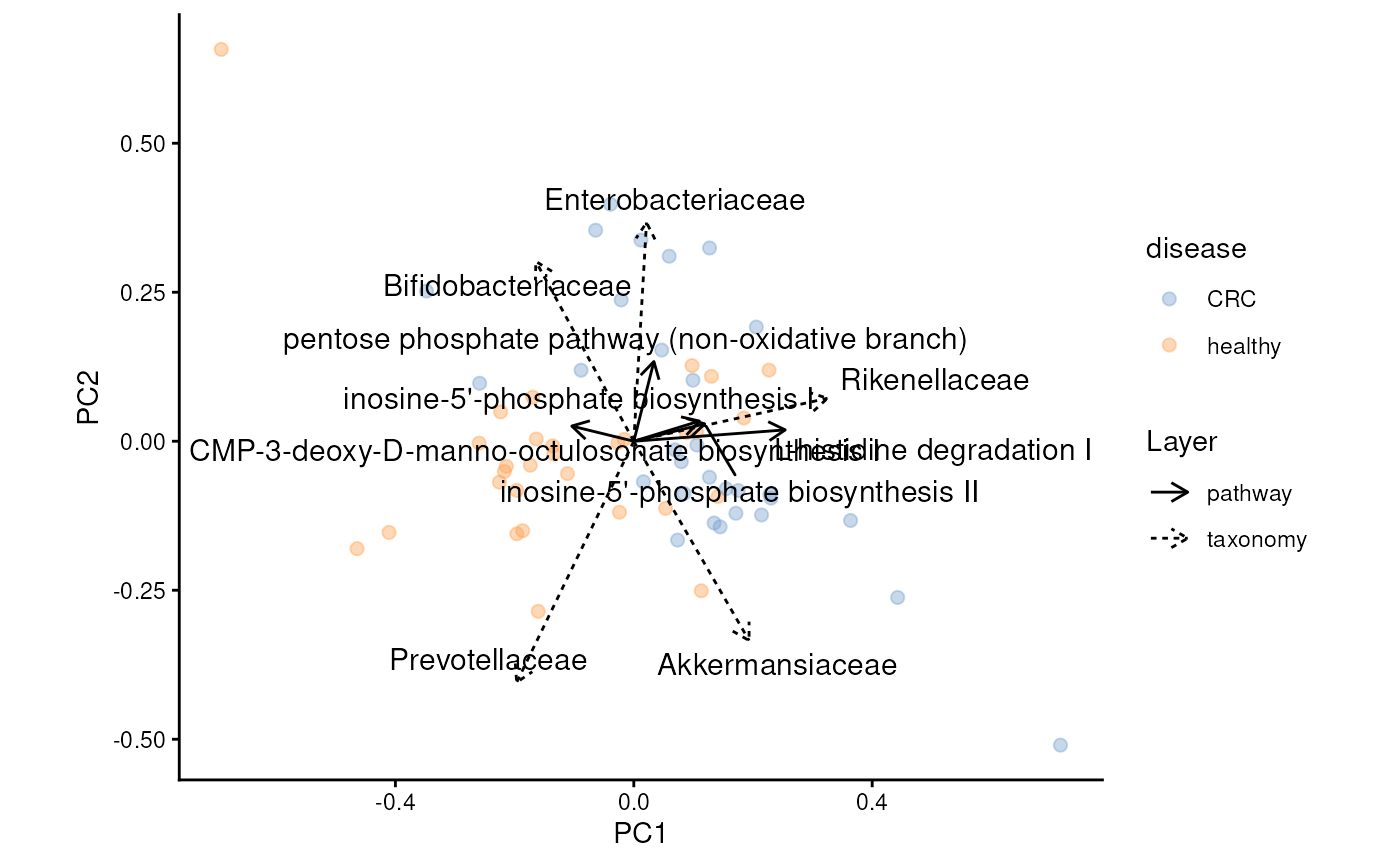
IntegratedLearner
Machine-learning applications often use a single data table, but different omics layers can contain complementary information that may improve prediction. There are three common strategies for integrating multiple layers:
Early fusion: Concatenate the different data tables into a single table and train one machine-learning model on the combined features.
Late fusion: Train a separate model for each omics layer and combine their predictions, for example by averaging or weighting them.
Intermediate fusion: Train separate models for each omics layer and then use a meta-model to combine the information or predictions from these models. This approach can often capture complementary information more flexibly than simple early or late fusion.
IntegratedLearner (Mallick et al. 2023) is an R package designed to facilitate multi-omics machine-learning and prediction. It can be used not only to build predictive models from multiple omics layers but also to identify features or biomarkers that contribute to prediction, helping determine which taxa, pathways, or other molecular features are most informative for the outcome.
library(IntegratedLearner)
model <- IntegratedLearner(
    MAE_train = mae,
    experiment = c(1, 2),
    assay.type = c("counts", "relative_abundance"),
    outcome_col = "disease",
    base_learner = "SL.randomForest",
    subject_id_col = "subject_id",
    family = binomial()
)
#> Time for model fit : 0.073 minutes
#> ========================================
#> Model fit for individual layers: SL.randomForest
#> Model fit for stacked layer: sl_nnls_auc
#> Model fit for concatenated layer: SL.randomForest
#> ========================================
#> AUC metric for training data:
#> Individual layers:
#>  pathway taxonomy
#>    0.921    0.949
#> ======================
#> Stacked model:0.948
#> ======================
#> Concatenated model:0.934
#> ======================
#> ========================================
#> Weights for individual layers predictions in IntegratedLearner:
#>  pathway taxonomy
#>    0.165    0.835
#> ========================================
Other integration approaches
Methods for integrating multi-omics data are rapidly evolving, and several other approaches are available depending on the research question.
Anansi uses guided pairwise association testing, where only feature pairs supported by prior biological knowledge or the literature are tested. This can improve interpretability by focusing on biologically plausible associations (Bastiaanssen et al. 2023).
Multi-Omics Factor Analysis (MOFA) identifies latent factors that capture shared and layer-specific sources of variation across multiple omics datasets. This can help reveal biological patterns that are common across data layers (Argelaguet et al. 2020).
DIABLO, implemented in mixOmics, uses partial least squares discriminant analysis (PLS-DA) to integrate multiple omics layers and identify features that are jointly informative for distinguishing predefined groups, making it particularly useful for biomarker discovery (Rohart et al. 2017).
The first two approaches, Anansi and MOFA, already support
MAE. Support for mixOmics/DIABLO is planned for a future
release.
Thank you for your time!
Join us!
OMA book: bioconductor.org/books/release/OMA/
Discussion forums: Bioconductor Zulip
Microbiome working group

Session information
sessionInfo()
#> R version 4.6.1 (2026-06-24)
#> Platform: x86_64-pc-linux-gnu
#> Running under: Ubuntu 24.04.4 LTS
#>
#> Matrix products: default
#> BLAS:   /usr/lib/x86_64-linux-gnu/openblas-pthread/libblas.so.3
#> LAPACK: /usr/lib/x86_64-linux-gnu/openblas-pthread/libopenblasp-r0.3.26.so;  LAPACK version 3.12.0
#>
#> locale:
#>  [1] LC_CTYPE=en_US.UTF-8       LC_NUMERIC=C
#>  [3] LC_TIME=en_US.UTF-8        LC_COLLATE=en_US.UTF-8
#>  [5] LC_MONETARY=en_US.UTF-8    LC_MESSAGES=en_US.UTF-8
#>  [7] LC_PAPER=en_US.UTF-8       LC_NAME=C
#>  [9] LC_ADDRESS=C               LC_TELEPHONE=C
#> [11] LC_MEASUREMENT=en_US.UTF-8 LC_IDENTIFICATION=C
#>
#> time zone: Etc/UTC
#> tzcode source: system (glibc)
#>
#> attached base packages:
#> [1] stats4    stats     graphics  grDevices utils     datasets  methods
#> [8] base
#>
#> other attached packages:
#>  [1] nnls_1.6                        IntegratedLearner_0.99.3
#>  [3] multiomics_0.99.0               knitr_1.52
#>  [5] maaslin3_1.5.7                  daa_0.99.0
#>  [7] miaViz_1.21.6                   ggraph_2.2.2
#>  [9] ggplot2_4.0.3                   mia_1.21.11
#> [11] TreeSummarizedExperiment_2.21.0 Biostrings_2.81.9
#> [13] XVector_0.53.0                  SingleCellExperiment_1.35.2
#> [15] MultiAssayExperiment_1.39.1     SummarizedExperiment_1.43.0
#> [17] Biobase_2.73.2                  GenomicRanges_1.65.4
#> [19] Seqinfo_1.3.2                   IRanges_2.47.5
#> [21] S4Vectors_0.51.10               BiocGenerics_0.59.12
#> [23] generics_0.1.4                  MatrixGenerics_1.25.0
#> [25] matrixStats_1.5.0               ape_5.8-1
#>
#> loaded via a namespace (and not attached):
#>   [1] nnet_7.3-21                 TH.data_1.1-5
#>   [3] vctrs_0.7.3                 digest_0.6.39
#>   [5] shape_1.4.6.1               BiocBaseUtils_1.15.1
#>   [7] ggrepel_0.9.8               parallelly_1.48.0
#>   [9] permute_0.9-10              MASS_7.3-66
#>  [11] fontLiberation_0.1.0        pkgdown_2.2.1
#>  [13] reshape2_1.4.5              foreach_1.5.2
#>  [15] withr_3.0.3                 xfun_0.61
#>  [17] ggfun_0.2.1                 survival_3.8-12
#>  [19] memoise_2.0.1               ggbeeswarm_0.7.3
#>  [21] MatrixModels_0.5-4          mixtools_2.0.0.1
#>  [23] systemfonts_1.3.2           ragg_1.5.2
#>  [25] tidytree_0.4.8              zoo_1.9-1
#>  [27] Formula_1.2-6               otel_0.2.0
#>  [29] httr_1.4.9                  rstatix_1.1.0
#>  [31] globals_0.19.1              nanonext_1.10.3
#>  [33] SuperLearner_2.0-42         rstudioapi_0.19.0
#>  [35] pan_2.0                     base64enc_0.1-6
#>  [37] ScaledMatrix_1.21.0         randomForest_4.7-1.2
#>  [39] polyclip_1.10-7             statip_0.2.3
#>  [41] SparseArray_1.13.4          stringr_1.6.0
#>  [43] desc_1.4.3                  rms_8.1-1
#>  [45] evaluate_1.0.5              S4Arrays_1.13.2
#>  [47] MiRKAT_1.2.3                glmnet_5.1
#>  [49] irlba_2.3.7                 colorspace_2.1-3
#>  [51] ROCR_1.0-12                 magrittr_2.0.5
#>  [53] viridis_0.6.5               ggtree_4.3.0
#>  [55] lattice_0.23-1              future.apply_1.20.2
#>  [57] SparseM_1.84-2              DECIPHER_3.9.3
#>  [59] gam_1.22-7                  scuttle_1.23.2
#>  [61] class_7.3-24                Hmisc_5.3-0
#>  [63] pillar_1.11.1               nlme_3.1-171
#>  [65] iterators_1.0.14            decontam_1.33.0
#>  [67] compiler_4.6.1              beachmat_2.29.3
#>  [69] stringi_1.8.9               gower_1.0.2
#>  [71] jomo_2.7-6                  lubridate_1.9.5
#>  [73] tokenizers_0.3.0            stabledist_0.7-2
#>  [75] minqa_1.2.8                 plyr_1.8.9
#>  [77] crayon_1.5.3                abind_1.4-8
#>  [79] scater_1.41.2               timeSeries_4052.112
#>  [81] gridGraphics_0.5-1          graphlayouts_1.2.5
#>  [83] sandwich_3.1-3              dplyr_1.2.1
#>  [85] codetools_0.2-20            multcomp_1.4-32
#>  [87] textshaping_1.0.5           recipes_1.4.0
#>  [89] BiocSingular_1.29.1         bslib_0.12.0
#>  [91] plotly_4.12.1               tidytext_0.4.3
#>  [93] ggvegan_0.2.1               splines_4.6.1
#>  [95] Rcpp_1.1.2                  quantreg_6.1
#>  [97] sparseMatrixStats_1.25.0    utf8_1.2.6
#>  [99] clue_0.3-68                 lme4_2.0-6
#> [101] fBasics_4052.98             fs_2.1.0
#> [103] listenv_1.1.0               checkmate_2.3.4
#> [105] DelayedMatrixStats_1.35.0   Rdpack_2.6.6
#> [107] PearsonDS_1.3.2             ggplotify_0.1.3
#> [109] tibble_3.3.1                Matrix_1.7-6
#> [111] statmod_1.5.2               tweenr_2.0.3
#> [113] pkgconfig_2.0.3             tools_4.6.1
#> [115] cachem_1.1.0                rbibutils_2.4.1
#> [117] viridisLite_0.4.3           DBI_1.3.0
#> [119] rmutil_1.1.10               fastmap_1.2.0
#> [121] rmarkdown_2.32              scales_1.4.0
#> [123] grid_4.6.1                  broom_1.0.13
#> [125] sass_0.4.10                 stable_1.1.7
#> [127] patchwork_1.3.2             BiocManager_1.30.27
#> [129] carData_3.0-6               rpart_4.1.27
#> [131] farver_2.1.2                reformulas_0.4.4
#> [133] tidygraph_1.3.1             mgcv_1.9-4
#> [135] yaml_2.3.12                 spatial_7.3-19
#> [137] foreign_0.8-91              cli_3.6.6
#> [139] purrr_1.2.2                 lifecycle_1.0.5
#> [141] caret_7.0-1                 mvtnorm_1.4-2
#> [143] bluster_1.23.1              lava_1.9.3
#> [145] kernlab_0.9-33              backports_1.5.1
#> [147] mirai_2.7.3                 modeest_2.5.0
#> [149] BiocParallel_1.47.0         timechange_0.4.0
#> [151] gtable_0.3.6                pROC_1.19.1
#> [153] parallel_4.6.1              SnowballC_0.7.1
#> [155] limma_3.99.0                jsonlite_2.0.0
#> [157] mitml_0.4-5                 yulab.utils_0.2.5
#> [159] vegan_2.7-6                 BiocNeighbors_2.7.3
#> [161] ranger_0.18.0               janeaustenr_1.0.0
#> [163] mice_3.19.0                 jquerylib_0.1.4
#> [165] polspline_1.1.25            segmented_2.2-2
#> [167] timeDate_4052.112           lazyeval_0.2.3
#> [169] htmltools_0.5.9             collapse_2.1.8
#> [171] rappdirs_0.3.4              glue_1.8.1
#> [173] optparse_1.8.2              gdtools_0.5.1
#> [175] treeio_1.37.1               gridExtra_2.3.1
#> [177] boot_1.3-32                 igraph_2.3.4
#> [179] R6_2.6.1                    tidyr_1.3.2
#> [181] ggiraph_0.9.6               CompQuadForm_1.4.4
#> [183] labeling_0.4.3              cluster_2.1.8.3
#> [185] aplot_0.3.2                 ipred_0.9-16
#> [187] nloptr_2.2.1                DirichletMultinomial_1.55.1
#> [189] DelayedArray_0.39.8         tidyselect_1.2.1
#> [191] vipor_0.4.7                 htmlTable_2.5.0
#> [193] ggforce_0.5.0               operator.tools_1.6.3.1
#> [195] inline_0.3.21               fontBitstreamVera_0.1.1
#> [197] car_3.1-5                   future_1.76.0
#> [199] ModelMetrics_1.2.2.2        GUniFrac_1.9
#> [201] rsvd_1.0.5                  S7_0.2.2
#> [203] BiocStyle_2.41.0            fontquiver_0.2.1
#> [205] data.table_1.18.6.1         htmlwidgets_1.6.4
#> [207] RColorBrewer_1.1-3          rlang_1.3.0
#> [209] logistf_1.26.1              formula.tools_1.7.1
#> [211] ggnewscale_0.5.2            hardhat_1.4.3
#> [213] beeswarm_0.4.0              prodlim_2026.03.11
References
University of Turku, tvborm@utu.fi↩︎