
Importing data into TreeSummarizedExperiment
Last updated on 2026-10-20 | Edit this page
Overview
Questions
- How do we load microbiome data into R?
- Why do we store the data in a single object?
- What is in our study data?
Objectives
- Create a
TreeSummarizedExperimentobject from an abundance table, a taxonomy table, sample information and a tree. - Access the abundance table, the taxonomy and the sample information of the object.
- Select a subset of the samples.
- Plot how many samples are in each study group.
Where are we?
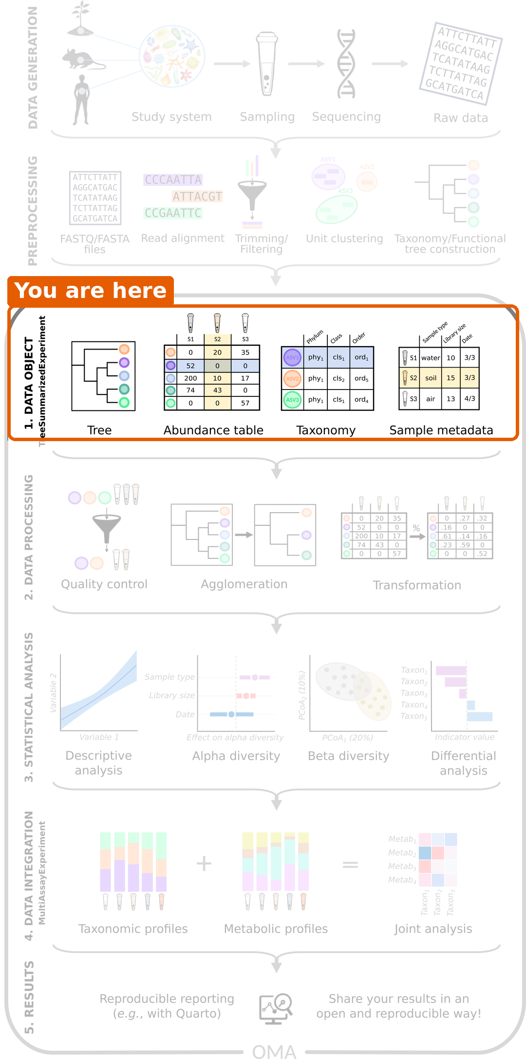
The sequencing reads of our study have already been turned into tables. In this episode, we bring these tables into R and combine them into a single data object. All later steps start from this object.
Load packages
R
library(mia)
library(miaViz)
Read the data files
We start by reading the four files from episode 3 into R. The first column of each CSV
file contains the row names, so we use row.names = 1.
R
counts  <- read.csv(file.path("data", "taxonomy_abundance.csv"), row.names = 1)
taxa    <- read.csv(file.path("data", "taxonomy_table.csv"), row.names = 1)
samples <- read.csv(file.path("data", "sample_metadata.csv"), row.names = 1)
tree    <- ape::read.tree(file.path("data", "phylogeny.tree"))
Let’s take a quick look at each of them. The abundance table has one
row per taxon and one column per sample. The row names start with the
taxonomic rank of the taxon, such as species-, and the
column names are sample IDs:
R
dim(counts)
OUTPUT
[1] 308 60R
counts[1:3, 1:3]
OUTPUT
                                      GupDM_A_11 GupDM_A_15 GupDM_A1
species-Escherichia_coli                 1632336    5666898  6814491
species-Alistipes_putredinis              964884          0   225222
species-Porphyromonas_asaccharolytica     463162          0    92810
The taxonomy table has one row per taxon:
R
head(taxa, n = 3)
OUTPUT
                                      superkingdom         phylum
species-Escherichia_coli                  Bacteria Proteobacteria
species-Alistipes_putredinis              Bacteria   Bacteroidota
species-Porphyromonas_asaccharolytica     Bacteria   Bacteroidota
                                                    class            order
species-Escherichia_coli              Gammaproteobacteria Enterobacterales
species-Alistipes_putredinis                  Bacteroidia    Bacteroidales
species-Porphyromonas_asaccharolytica         Bacteroidia    Bacteroidales
                                                  family         genus
species-Escherichia_coli              Enterobacteriaceae   Escherichia
species-Alistipes_putredinis               Rikenellaceae     Alistipes
species-Porphyromonas_asaccharolytica Porphyromonadaceae Porphyromonas
                                                            species
species-Escherichia_coli                           Escherichia coli
species-Alistipes_putredinis                   Alistipes putredinis
species-Porphyromonas_asaccharolytica Porphyromonas asaccharolytica
The sample information has one row per sample:
R
samples[1:3, c("disease", "age", "gender", "location")]
OUTPUT
           disease age gender location
GupDM_A_11     CRC  41 female   Kerala
GupDM_A_15     CRC  59   male   Kerala
GupDM_A1       CRC  62   male   Kerala
And the tree connects the taxa:
R
tree
OUTPUT
Phylogenetic tree with 10430 tips and 10429 internal nodes.

Tip labels:
  k__Archaea|p__Candidatus_Micrarchaeota|c__Candidatus_Micrarchaeota_unclassified|o__Candidatus_Micrarchaeota_unclassified|f__Candidatus_Micrarchaeota_unclassified|g__Candidatus_Micrarchaeota_unclassified|s__Candidatus_Micrarchaeota_archaeon_CG1_02_55_22, k__Archaea|p__Archaea_unclassified|c__Archaea_unclassified|o__Archaea_unclassified|f__Archaea_unclassified|g__Archaea_unclassified|s__archaeon_GW2011_AR15, k__Archaea|p__Candidatus_Diapherotrites|c__Candidatus_Diapherotrites_unclassified|o__Candidatus_Diapherotrites_unclassified|f__Candidatus_Diapherotrites_unclassified|g__Candidatus_Diapherotrites_unclassified|s__Candidatus_Diapherotrites_archaeon_CG08_land_8_20_14_0_20_34_12, k__Archaea|p__Archaea_unclassified|c__Archaea_unclassified|o__Archaea_unclassified|f__Archaea_unclassified|g__Archaea_unclassified|s__archaeon_GW2011_AR10, k__Archaea|p__Candidatus_Diapherotrites|c__Candidatus_Diapherotrites_unclassified|o__Candidatus_Diapherotrites_unclassified|f__Candidatus_Diapherotrites_unclassified|g__Candidatus_Diapherotrites_unclassified|s__Candidatus_Diapherotrites_archaeon_CG11_big_fil_rev_8_21_14_0_20_37_9, k__Archaea|p__Euryarchaeota|c__Euryarchaeota_unclassified|o__Euryarchaeota_unclassified|f__Euryarchaeota_unclassified|g__Euryarchaeota_unclassified|s__Euryarchaeota_archaeon_TMED173, ...

Rooted; includes branch length(s).
The tree is a reference tree from MetaPhlAn, the tool that produced our tables. It contains 10430 species, many more than the 308 in our data. That is fine: each of our taxa has a tip with the same name in the tree, and this is how R knows which tip belongs to which taxon. The printout shows the first few tip labels, which belong to species that are not in our data.
Why put everything into one object?
We now have four separate objects that describe the same data. This is risky: if we remove a sample from the abundance table, we have to remember to remove it from the sample information too. If we forget, the tables no longer match, and our results will be wrong without any warning.
The solution is to store everything in a single object that keeps the
parts in sync. In Bioconductor, microbiome data is stored in a
TreeSummarizedExperiment (TreeSE for
short).
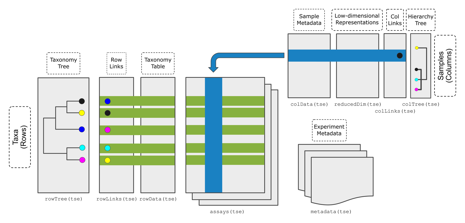
Figure: the TreeSummarizedExperiment class (Huang et al. 2021, F1000Research). Source: OMA.
The figure shows all the parts a TreeSE can hold. In this lesson, we only need these four:
| Part | Contains | In our data |
|---|---|---|
assays |
The abundance tables. Rows are taxa, columns are samples. | Read counts |
rowData |
Information about the rows (taxa) | Taxonomy |
colData |
Information about the columns (samples) | Disease, age, gender, location, … |
rowTree |
A tree that connects the rows | Phylogenetic tree |
TreeSE and SummarizedExperiment
If you have used the SummarizedExperiment class before,
for example in the Introduction
to data analysis with R and Bioconductor lesson: a TreeSE is a
SummarizedExperiment with extra room for trees. Everything
you know about SummarizedExperiment also works for TreeSE.
The only difference in our data is what the rows are: genes in that
lesson, taxa here. The functions assay(),
rowData() and colData() and subsetting with
[ , ] work exactly as you learned there.
Create the TreeSE
We combine the four parts with the function
TreeSummarizedExperiment(). The abundance table must be a
matrix, so we convert it with as.matrix(). We also give the
data a name with mainExpName. This becomes useful in the
bonus section of the next episode, where we store the data at several
taxonomic ranks in the same object.
R
tse <- TreeSummarizedExperiment(
    assays  = list(counts = as.matrix(counts)),
    rowData = taxa,
    colData = samples,
    rowTree = tree,
    mainExpName = "main"
)
tse
OUTPUT
class: TreeSummarizedExperiment
dim: 308 60
metadata(0):
assays(1): counts
rownames(308): species-Escherichia_coli species-Alistipes_putredinis
  ... species-Campylobacter_ureolyticus
  species-Prevotella_sp._oral_taxon_376
rowData names(7): superkingdom phylum ... genus species
colnames(60): GupDM_A_11 GupDM_A_15 ... GupDM_JO GupDM_JP
colData names(27): study_name subject_id ... disease_stage
  disease_location
reducedDimNames(0):
mainExpName: main
altExpNames(0):
rowLinks: a LinkDataFrame (308 rows)
rowTree: 1 phylo tree(s) (10430 leaves)
colLinks: NULL
colTree: NULL
The printout summarizes the object:
-
dim: 308 taxa (rows) and 60 samples (columns). -
assays(1): counts: one abundance table, namedcounts. -
rowData names(7): the taxonomy columns. -
colData names(27): the columns of sample information. -
rowTree: the phylogenetic tree.
Look inside the TreeSE
Each part has its own accessor function.
The abundance table is accessed with assay():
R
assay(tse, "counts")[1:3, 1:3]
OUTPUT
                                      GupDM_A_11 GupDM_A_15 GupDM_A1
species-Escherichia_coli                 1632336    5666898  6814491
species-Alistipes_putredinis              964884          0   225222
species-Porphyromonas_asaccharolytica     463162          0    92810
The taxonomy is accessed with rowData():
R
rowData(tse)
OUTPUT
DataFrame with 308 rows and 7 columns
                                      superkingdom         phylum
                                       <character>    <character>
species-Escherichia_coli                  Bacteria Proteobacteria
species-Alistipes_putredinis              Bacteria   Bacteroidota
species-Porphyromonas_asaccharolytica     Bacteria   Bacteroidota
species-Bacteroides_uniformis             Bacteria   Bacteroidota
species-Prevotella_stercorea              Bacteria   Bacteroidota
...                                            ...            ...
species-Ruminococcus_obeum_CAG-39         Bacteria     Firmicutes
species-Streptococcus_lutetiensis         Bacteria     Firmicutes
species-Prevotella_timonensis             Bacteria   Bacteroidota
species-Campylobacter_ureolyticus         Bacteria Proteobacteria
species-Prevotella_sp._oral_taxon_376     Bacteria   Bacteroidota
                                                      class             order
                                                <character>       <character>
species-Escherichia_coli                Gammaproteobacteria  Enterobacterales
species-Alistipes_putredinis                    Bacteroidia     Bacteroidales
species-Porphyromonas_asaccharolytica           Bacteroidia     Bacteroidales
species-Bacteroides_uniformis                   Bacteroidia     Bacteroidales
species-Prevotella_stercorea                    Bacteroidia     Bacteroidales
...                                                     ...               ...
species-Ruminococcus_obeum_CAG-39                Clostridia     Eubacteriales
species-Streptococcus_lutetiensis                   Bacilli   Lactobacillales
species-Prevotella_timonensis                   Bacteroidia     Bacteroidales
species-Campylobacter_ureolyticus     Epsilonproteobacteria Campylobacterales
species-Prevotella_sp._oral_taxon_376           Bacteroidia     Bacteroidales
                                                  family         genus
                                             <character>   <character>
species-Escherichia_coli              Enterobacteriaceae   Escherichia
species-Alistipes_putredinis               Rikenellaceae     Alistipes
species-Porphyromonas_asaccharolytica Porphyromonadaceae Porphyromonas
species-Bacteroides_uniformis             Bacteroidaceae   Bacteroides
species-Prevotella_stercorea              Prevotellaceae    Prevotella
...                                                  ...           ...
species-Ruminococcus_obeum_CAG-39       Oscillospiraceae  Ruminococcus
species-Streptococcus_lutetiensis       Streptococcaceae Streptococcus
species-Prevotella_timonensis             Prevotellaceae    Prevotella
species-Campylobacter_ureolyticus     Campylobacteraceae Campylobacter
species-Prevotella_sp._oral_taxon_376     Prevotellaceae    Prevotella
                                                     species
                                                 <character>
species-Escherichia_coli                    Escherichia coli
species-Alistipes_putredinis            Alistipes putredinis
species-Porphyromonas_asaccharolytica Porphyromonas asacch..
species-Bacteroides_uniformis          Bacteroides uniformis
species-Prevotella_stercorea            Prevotella stercorea
...                                                      ...
species-Ruminococcus_obeum_CAG-39     Ruminococcus obeum C..
species-Streptococcus_lutetiensis     Streptococcus luteti..
species-Prevotella_timonensis          Prevotella timonensis
species-Campylobacter_ureolyticus     Campylobacter ureoly..
species-Prevotella_sp._oral_taxon_376 Prevotella sp. oral ..
The sample information is accessed with colData():
R
colData(tse)
OUTPUT
DataFrame with 60 rows and 27 columns
            study_name  subject_id   body_site antibiotics_current_use
           <character> <character> <character>             <character>
GupDM_A_11 GuptaA_2019   GupDM_A11       stool                      no
GupDM_A_15 GuptaA_2019   GupDM_A15       stool                      no
GupDM_A1   GuptaA_2019    GupDM_A1       stool                      no
GupDM_A10  GuptaA_2019   GupDM_A10       stool                      no
GupDM_A12  GuptaA_2019   GupDM_A12       stool                      no
...                ...         ...         ...                     ...
GupDM_JL   GuptaA_2019    GupDM_JL       stool                      no
GupDM_JM   GuptaA_2019    GupDM_JM       stool                      no
GupDM_JN   GuptaA_2019    GupDM_JN       stool                      no
GupDM_JO   GuptaA_2019    GupDM_JO       stool                      no
GupDM_JP   GuptaA_2019    GupDM_JP       stool                      no
           study_condition     disease       age age_category      gender
               <character> <character> <integer>  <character> <character>
GupDM_A_11             CRC         CRC        41        adult      female
GupDM_A_15             CRC         CRC        59        adult        male
GupDM_A1               CRC         CRC        62        adult        male
GupDM_A10              CRC         CRC        65        adult      female
GupDM_A12              CRC         CRC        65        adult        male
...                    ...         ...       ...          ...         ...
GupDM_JL               CRC         CRC        59        adult      female
GupDM_JM               CRC         CRC        60        adult        male
GupDM_JN               CRC         CRC        58        adult        male
GupDM_JO               CRC         CRC        71       senior        male
GupDM_JP               CRC         CRC        67       senior        male
               country    location non_westernized sequencing_platform
           <character> <character>     <character>         <character>
GupDM_A_11         IND      Kerala              no     IlluminaNextSeq
GupDM_A_15         IND      Kerala              no     IlluminaNextSeq
GupDM_A1           IND      Kerala              no     IlluminaNextSeq
GupDM_A10          IND      Kerala              no     IlluminaNextSeq
GupDM_A12          IND      Kerala              no     IlluminaNextSeq
...                ...         ...             ...                 ...
GupDM_JL           IND      Bhopal              no     IlluminaNextSeq
GupDM_JM           IND      Bhopal              no     IlluminaNextSeq
GupDM_JN           IND      Bhopal              no     IlluminaNextSeq
GupDM_JO           IND      Bhopal              no     IlluminaNextSeq
GupDM_JP           IND      Bhopal              no     IlluminaNextSeq
           DNA_extraction_kit      PMID number_reads number_bases
                  <character> <integer>    <integer>    <numeric>
GupDM_A_11             Qiagen  31719139      6227234    883347281
GupDM_A_15             Qiagen  31719139      9884266   1384530792
GupDM_A1               Qiagen  31719139     27687226   3808647004
GupDM_A10              Qiagen  31719139      8468208   1174245166
GupDM_A12              Qiagen  31719139      6988838    984235167
...                       ...       ...          ...          ...
GupDM_JL               Qiagen  31719139      9878044   1387793557
GupDM_JM               Qiagen  31719139     10328094   1435043694
GupDM_JN               Qiagen  31719139      9789278   1347588954
GupDM_JO               Qiagen  31719139     11274338   1501226163
GupDM_JP               Qiagen  31719139     10400668   1428270555
           minimum_read_length median_read_length NCBI_accession
                     <integer>          <integer>    <character>
GupDM_A_11                  60                151     SRR8865600
GupDM_A_15                  60                150     SRR8865596
GupDM_A1                    60                150     SRR8865598
GupDM_A10                   60                150     SRR8865599
GupDM_A12                   60                150     SRR8865601
...                        ...                ...            ...
GupDM_JL                    60                151     SRR8865572
GupDM_JM                    60                150     SRR8865575
GupDM_JN                    60                150     SRR8865574
GupDM_JO                    60                150     SRR8865581
GupDM_JP                    60                150     SRR8865580
                          curator       BMI disease_subtype         tnm
                      <character> <numeric>     <character> <character>
GupDM_A_11 Arianna_Bonetti;Paol..     19.22  adenocarcinoma      t2m0n0
GupDM_A_15 Arianna_Bonetti;Paol..     21.40  adenocarcinoma      t2n0m0
GupDM_A1   Arianna_Bonetti;Paol..     20.08  adenocarcinoma      t2n0m0
GupDM_A10  Arianna_Bonetti;Paol..     21.01  adenocarcinoma      t3n2m0
GupDM_A12  Arianna_Bonetti;Paol..     20.32  adenocarcinoma      t2n2m0
...                           ...       ...             ...         ...
GupDM_JL   Arianna_Bonetti;Paol..     20.34  adenocarcinoma      t4n1m0
GupDM_JM   Arianna_Bonetti;Paol..     18.33  adenocarcinoma      t2n0m0
GupDM_JN   Arianna_Bonetti;Paol..     19.92  adenocarcinoma      t2n0m0
GupDM_JO   Arianna_Bonetti;Paol..     20.03  adenocarcinoma      t4n1m0
GupDM_JP   Arianna_Bonetti;Paol..     17.69  adenocarcinoma      t3n2m0
                  fobt disease_stage disease_location
           <character>   <character>      <character>
GupDM_A_11         yes             I           rectum
GupDM_A_15         yes             I           rectum
GupDM_A1           yes             I           rectum
GupDM_A10          yes           III            colon
GupDM_A12          yes           III           rectum
...                ...           ...              ...
GupDM_JL           yes           III           rectum
GupDM_JM           yes             I           rectum
GupDM_JN           yes             I           rectum
GupDM_JO           yes           III    sigmoid_colon
GupDM_JP           yes           III           rectum
A single column of the sample information can be accessed with
$, just as in a data frame:
R
table(tse$disease)
OUTPUT
    CRC healthy
     30      30
rowData() and colData() return a
DataFrame, the Bioconductor version of a data frame. It
works like a data.frame, but prints only the first and last
rows. The tree is accessed with rowTree(tse). We do not
need to look at it now: functions that use the tree, such as
phylogenetic diversity in episode
6, find it there on their own.
Challenge 1: Where is the information?
In which part of tse would you find the age of each
person?
assay(tse, "counts")rowData(tse)colData(tse)rowTree(tse)
-
colData(tse). Age describes a sample (a person), and information about samples is stored incolData. You can get the ages withtse$age.
Challenge 2: Which phylum?
Find out which phylum the first taxon in tse belongs
to.
Hint: the taxonomy is in rowData(tse), and its
columns are named superkingdom, phylum,
class, …
R
rownames(tse)[1]
OUTPUT
[1] "species-Escherichia_coli"R
rowData(tse)$phylum[1]
OUTPUT
[1] "Proteobacteria"Select a subset of samples
A TreeSE can be subset with square brackets
[rows, columns], just like a data frame. Rows are taxa and
columns are samples. To keep only the samples from people with CRC, we
select the columns where disease is "CRC":
R
tse_crc <- tse[, tse$disease == "CRC"]
tse_crc
OUTPUT
class: TreeSummarizedExperiment
dim: 308 30
metadata(0):
assays(1): counts
rownames(308): species-Escherichia_coli species-Alistipes_putredinis
  ... species-Campylobacter_ureolyticus
  species-Prevotella_sp._oral_taxon_376
rowData names(7): superkingdom phylum ... genus species
colnames(30): GupDM_A_11 GupDM_A_15 ... GupDM_JO GupDM_JP
colData names(27): study_name subject_id ... disease_stage
  disease_location
reducedDimNames(0):
mainExpName: main
altExpNames(0):
rowLinks: a LinkDataFrame (308 rows)
rowTree: 1 phylo tree(s) (10430 leaves)
colLinks: NULL
colTree: NULL
Result: the new object has 30 samples. The abundance table and the sample information were subset together, so they still match. This is the main reason we use a TreeSE.
Challenge 3: Healthy people only
- Create an object
tse_healthythat contains only the samples from healthy people. - How many samples does it have?
R
tse_healthy <- tse[, tse$disease == "healthy"]
ncol(tse_healthy)
OUTPUT
[1] 30A first look at the study
Before any analysis, it is good to know who is in the study. The
miaViz function plotBarplot() counts the samples in each
group of a colData column (col.var):
R
plotBarplot(tse, col.var = "disease")
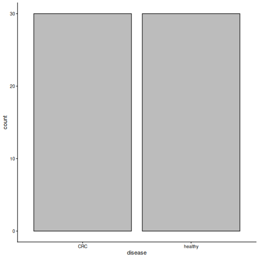
Result: the study has 30 people with CRC and 30 healthy people.
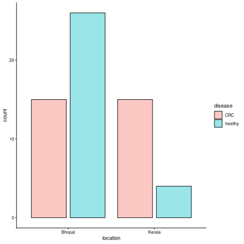
The people come from two places: the city of Bhopal and the state of
Kerala. With fill.by, we can colour the bars by a second
variable:
R
plotBarplot(tse, col.var = "location", fill.by = "disease")
Challenge 4: What do you notice?
Look at the plot above.
- From which location do most of the healthy people come?
- Suppose we find that the microbiome of CRC patients differs from that of healthy people. Why could this be a problem?
- Most healthy people come from Bhopal, while the CRC patients come
equally from both places. You can check the numbers with
table(tse$location, tse$disease). - Diet and lifestyle differ between the places, and they affect the gut microbiome. A difference between CRC and healthy people could therefore be partly a difference between the two places. We will take this into account in the episodes on beta diversity and differential abundance.
Save the object
We save the TreeSE so that we can load it again in the next episode, without repeating the import steps.
R
saveRDS(tse, file.path("data", "tse.rds"))
Importing your own data
In this lesson, we built the TreeSE from plain tables. Your own data probably comes from a tool such as QIIME 2, MetaPhlAn or mothur, or is stored as a phyloseq object. The mia package has functions that import these formats directly into a TreeSE. See the Import chapter of OMA.
- A
TreeSummarizedExperimentkeeps the abundance table, taxonomy, sample information and tree together and in sync. - Rows are taxa and columns are samples.
-
assay(),rowData()andcolData()access the abundance table, the taxonomy and the sample information. - Subsetting with
[rows, columns]keeps all parts of the object in sync. -
plotBarplot()gives a quick overview of the study groups. In our study, the groups differ in more than disease: most healthy people come from Bhopal.