Capstone: analyse a new dataset

Overview

Questions

• Can I run a complete microbiome analysis on my own?
• How do I report the results of a microbiome analysis?

Objectives

• Explore and prepare a new microbiome dataset.
• Compare alpha diversity, beta diversity and the abundance of single taxa between two groups, while taking a second variable into account.
• Interpret results that differ from those of the main study, including results that are not significant.
• Summarize an analysis in a short written report.

Where are we?

---

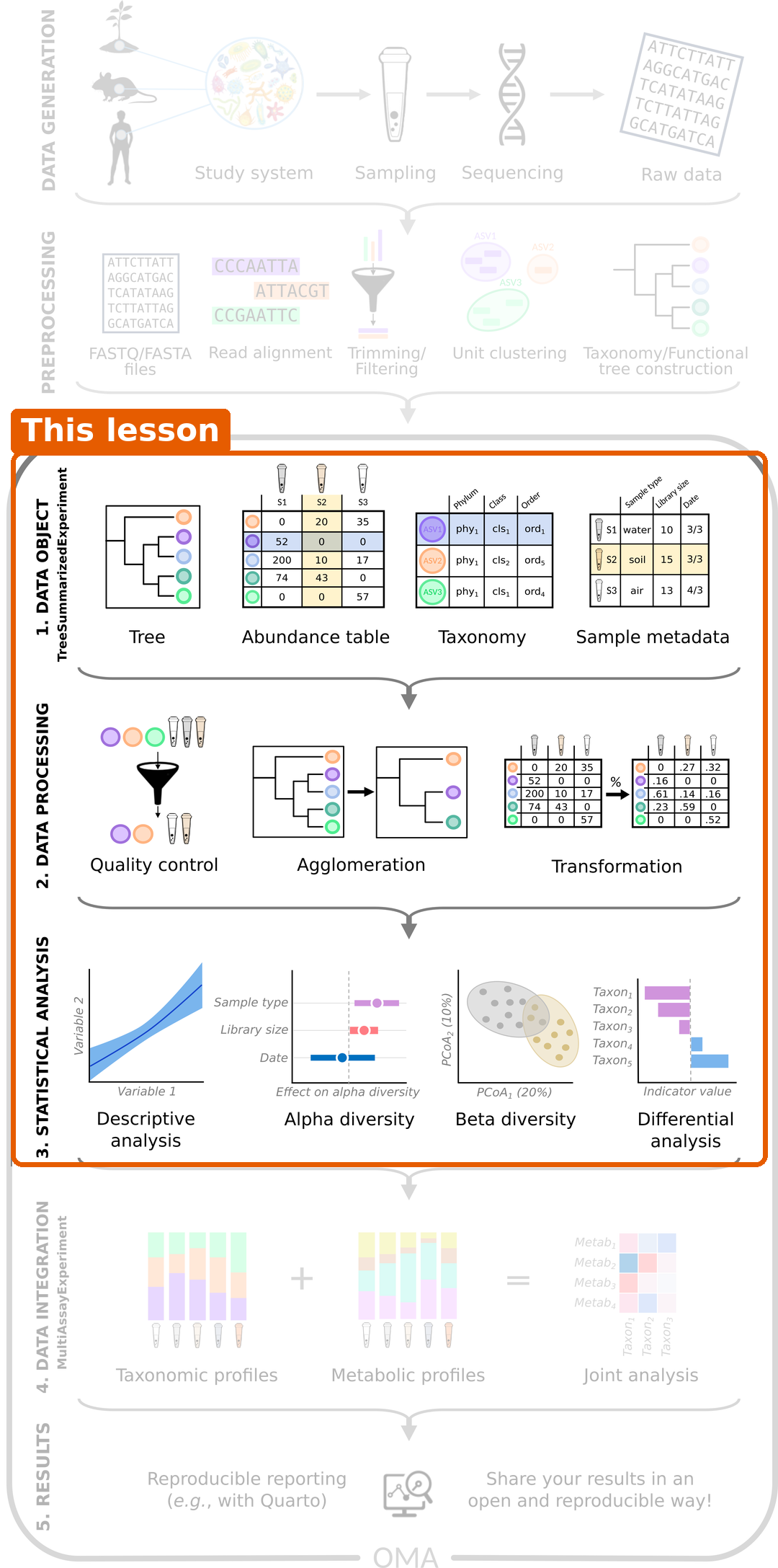
You now know every step of the workflow: import, exploration and preparation, alpha diversity, beta diversity and differential abundance. In this episode, you run the whole workflow on your own, on a dataset you have not seen before. The tasks below guide you. Try each task yourself before you open its solution, and use the earlier episodes as a reference.

Plan about 40 minutes for Tasks 1–5 and 10 minutes for the report in Task 7. Task 6 and the optional part of Task 3 are extras for those who have time. If you get stuck on a task, open its solution and continue: the report matters more than solving every task alone.

The dataset

---

The mia package includes several example datasets. We use Tengeler2020, from a study of attention deficit hyperactivity disorder (ADHD) (Tengeler et al. 2020). The researchers transferred gut microbiota from people with ADHD and from healthy controls into germ-free mice, to test whether the microbiota can affect the brain. The dataset holds 27 gut microbiota profiles. For each sample, we know:

• patient_status: whether the microbiota came from a person with ADHD or from a control;
• cohort: in which of three experimental cohorts the sample was processed.

Unlike our main study, these data come from 16S amplicon sequencing (episode 2). The table holds real read counts, and the taxa are genus-level groups of reads (for example Bacteroides_1, Bacteroides_2).

The research question is:

Does the gut microbiota of people with ADHD differ from that of controls, and which bacteria differ?

Load packages and data

---

R

library(mia)
library(miaViz)
library(maaslin3)

R

data("Tengeler2020", package = "mia")
tse <- Tengeler2020
tse

OUTPUT

class: TreeSummarizedExperiment
dim: 151 27
metadata(0):
assays(1): counts
rownames(151): Bacteroides Bacteroides_1 ... Parabacteroides_8
  Unidentified_Lachnospiraceae_14
rowData names(6): Kingdom Phylum ... Family Genus
colnames(27): A110 A12 ... A35 A38
colData names(4): patient_status cohort patient_status_vs_cohort
  sample_name
reducedDimNames(0):
mainExpName: NULL
altExpNames(0):
rowLinks: a LinkDataFrame (151 rows)
rowTree: 1 phylo tree(s) (151 leaves)
colLinks: NULL
colTree: NULL

The data is already a TreeSE, with a phylogenetic tree. Note that the taxonomic ranks in rowData are capitalized: Phylum, Family, Genus.

Challenge

Task 1: Who is in the study?

1. How many samples are there from ADHD donors and from controls?
2. How are the two groups spread over the three cohorts? Make a table and a bar plot.
3. Could the cohort be a confounder, as the location was in our main study?

Show me the solution

R

table(tse$patient_status, tse$cohort)

OUTPUT

          Cohort_1 Cohort_2 Cohort_3
  ADHD           4        5        4
  Control        6        5        3

R

plotBarplot(tse, col.var = "cohort", fill.by = "patient_status")

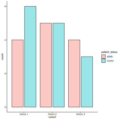
1. There are 13 ADHD samples and 14 control samples.
2. Every cohort has both ADHD and control samples, in roughly equal numbers.
3. The cohort is not strongly linked to the patient status, so it is a much smaller problem than the location was in the main study. Still, samples processed together can be more similar to each other (a batch effect), so it is good practice to include cohort in the models.

Challenge

Task 2: Explore and prepare the data

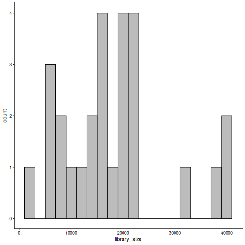
1. Calculate the library size of each sample, store it in colData, and plot it with plotHistogram(). How much do the library sizes differ?
2. Add relative abundances with transformAssay().
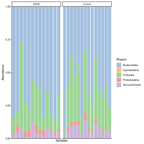
3. Plot the composition of each sample at phylum level, split by patient_status. Which phyla dominate?
4. Which five taxa are the most abundant?
5. Add rclr values with transformAssay(). Why do we add them only after the composition plot?

Show me the solution

R

tse$library_size <- colSums(assay(tse, "counts"))
summary(tse$library_size)

OUTPUT

   Min. 1st Qu.  Median    Mean 3rd Qu.    Max.
   1772   11804   16745   17997   21502   40584 

R

plotHistogram(tse, col.var = "library_size", binwidth = 2000)

R

tse <- transformAssay(tse, assay.type = "counts", method = "relabundance")

R

plotAbundance(
    tse, assay.type = "relabundance", group = "Phylum",
    col.var = "patient_status", facet.cols = TRUE, scales = "free_x"
)

R

getTop(tse, top = 5)

OUTPUT

[1] "Bacteroides"     "Bacteroides_1"   "Parabacteroides" "Bacteroides_2"
[5] "Akkermansia"    

R

tse <- transformAssay(tse, assay.type = "counts", method = "rclr")
assayNames(tse)

OUTPUT

[1] "counts"       "relabundance" "rclr"        

1. The largest library is about 23 times larger than the smallest. With real read counts, such differences matter for richness (see Task 3).
2. Bacteroidetes dominate (on average 65 % of the community), followed by Firmicutes (27 %) and Verrucomicrobia (6 %). By eye, the two groups look similar. This dataset uses the older phylum name Bacteroidetes for the phylum that is called Bacteroidota in our main study. plotAbundance() may warn about removed rows; as in episode 5, this is harmless.
3. Mostly Bacteroides groups, Parabacteroides and Akkermansia.
4. With group = "Phylum", plotAbundance() agglomerates all tables to phylum level, by summing. Summed rclr values are meaningless, and plotAbundance() would warn about them. Remember the rule from episode 5: agglomerate first, then transform.

Challenge

Task 3: Alpha diversity

1. Calculate observed richness, Shannon diversity and Faith’s phylogenetic diversity with addAlpha().
2. Plot the Shannon diversity by patient_status, and test the difference with the Wilcoxon test. Do the same for the other two indices.
3. Optional: this is amplicon data with real read counts, and the library sizes differ a lot. Calculate a rarefied richness with the sample and niter arguments of addAlpha() (rarefy to the smallest library size). Does the conclusion change?

Show me the solution

R

tse <- addAlpha(
    tse, assay.type = "counts",
    index = c("observed_richness", "shannon_diversity", "faith_diversity")
)

R

plotBoxplot(tse, col.var = "shannon_diversity", x = "patient_status")

R

p_shannon <- wilcox.test(shannon_diversity ~ patient_status, data = colData(tse))$p.value
p_richness <- wilcox.test(observed_richness ~ patient_status, data = colData(tse))$p.value
p_faith <- wilcox.test(faith_diversity ~ patient_status, data = colData(tse))$p.value
c(shannon = p_shannon, richness = p_richness, faith = p_faith)

OUTPUT

  shannon  richness     faith
0.4879480 0.9333796 0.9809717 

R

tse <- addAlpha(
    tse, assay.type = "counts", index = "observed_richness",
    sample = min(tse$library_size), niter = 10, name = "richness_rarefied"
)
p_rarefied <- wilcox.test(richness_rarefied ~ patient_status, data = colData(tse))$p.value
p_rarefied

OUTPUT

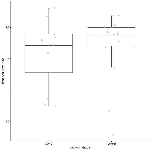
[1] 1

2. None of the indices differ between the groups (Shannon p = 0.49, richness p = 0.93, Faith p = 0.98).
3. The rarefied richness does not differ either (p = 1). The conclusion is the same. Rarefying makes the richness values comparable across samples with different sequencing depths, which is why it is common for amplicon data.

Challenge

Task 4: Beta diversity

1. Make a PCoA with Bray–Curtis dissimilarity, and colour it by patient_status. Then colour it by cohort.
2. Test with PERMANOVA whether the composition differs by patient_status, taking cohort into account (formula = x ~ patient_status + cohort). Add by = "margin", so that each variable is tested while the other is taken into account.
3. Check the homogeneity of the group spreads. Can you trust the PERMANOVA result?

Show me the solution

R

tse <- addMDS(
    tse, assay.type = "relabundance", method = "bray", name = "PCoA_BC"
)
plotOrdination(tse, "PCoA_BC", colour.by = "patient_status")

R

plotOrdination(tse, "PCoA_BC", colour.by = "cohort")

R

permanova <- getPERMANOVA(
    tse, assay.type = "relabundance", method = "bray",
    formula = x ~ patient_status + cohort, by = "margin"
)
permanova$permanova

OUTPUT

Permutation test for adonis under reduced model
Marginal effects of terms
Permutation: free
Number of permutations: 999

adonis2(formula = formula, data = data, method = ..1, by = by, na.action = na.action)
               Df SumOfSqs      R2      F Pr(>F)
patient_status  1   0.3790 0.06819 1.7880  0.104
cohort          2   0.3212 0.05780 0.7578  0.686
Residual       23   4.8748 0.87721
Total          26   5.5572 1.00000              

R

permanova$homogeneity

OUTPUT

               Df      Sum Sq      Mean Sq          F N.Perm Pr(>F)
patient_status  1 0.001208740 0.0012087403 0.08912270    999  0.754
cohort          2 0.001793416 0.0008967079 0.07260098    999  0.927
               Total variance Explained variance
patient_status      0.3402751        0.003552244
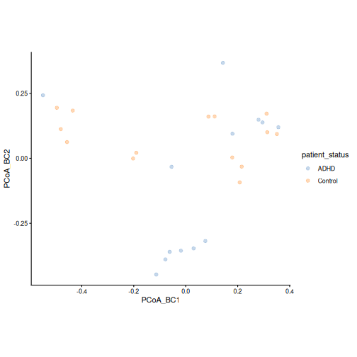
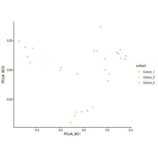
cohort              0.2982218        0.006013699

1. ADHD and control samples are found on both sides of the first axis, so the groups overlap a lot. A tight group of ADHD samples lies at the bottom of the plot; it contains samples from two cohorts. The cohorts are spread over the whole plot.
2. Patient status explains 7 % of the differences between samples, but this is not significant (p = 0.1). The cohort is not significant either (p = 0.69).
3. The spreads do not differ (p = 0.75), so the assumption of PERMANOVA holds. We find no significant difference in overall composition, even though some ADHD samples form their own group in the plot.

Challenge

Task 5: Differential abundance and prevalence

1. Make Control the reference level of patient_status, and turn cohort into a factor.
2. Keep the taxa with a relative abundance of at least 0.1 % in at least 10 % of the samples.
3. Run MaAsLin 3 with formula = ~ patient_status + cohort and output = "maaslin3_output_tengeler".
4. Which taxa differ in abundance between ADHD and controls (q < 0.05)? In which direction? Do any taxa differ in prevalence?
5. Plot the relative abundance of the taxa that differ in abundance by patient_status.

Show me the solution

R

tse$patient_status <- factor(tse$patient_status, levels = c("Control", "ADHD"))
tse$cohort <- factor(tse$cohort)
tse_prevalent <- subsetByPrevalent(
    tse, assay.type = "relabundance",
    detection = 0.001, prevalence = 0.1
)
nrow(tse_prevalent)

OUTPUT

[1] 145

R

fit <- maaslin3(
    tse_prevalent,
    formula = ~ patient_status + cohort,
    output = "maaslin3_output_tengeler",
    plot_summary_plot = FALSE,
    plot_associations = FALSE,
    verbosity = "ERROR"
)
res <- fit$fit_data_abundance$results
res <- res[res$metadata == "patient_status", ]
sig <- res[res$qval_individual < 0.05 & !is.na(res$qval_individual), ]
sig[, c("feature", "coef", "qval_individual")]

OUTPUT

            feature      coef qval_individual
1       Coprobacter  2.984114      0.01305400
2 Subdoligranulum_1 -2.378099      0.04089055

R

res_pa <- fit$fit_data_prevalence$results
res_pa <- res_pa[res_pa$metadata == "patient_status", ]
sig_pa <- res_pa[res_pa$qval_individual < 0.05 & !is.na(res_pa$qval_individual), ]
sig_pa[, c("feature", "coef", "qval_individual")]

OUTPUT

[1] feature         coef            qval_individual
<0 rows> (or 0-length row.names)

R

plotBoxplot(
    tse, assay.type = "relabundance", x = "patient_status",
    features = sig$feature, facet.by = "rownames"
)

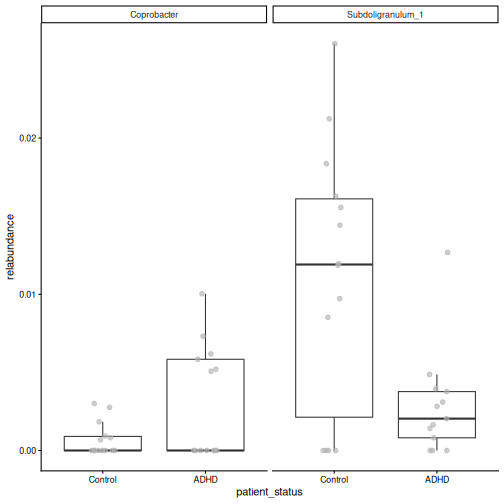
4. 2 of the 145 taxa differ in abundance. More abundant in ADHD: Coprobacter. Less abundant in ADHD: Subdoligranulum_1. 0 taxa differ in prevalence.
5. The box plots show the differences, but also a large overlap between the groups and many zeros. With only 27 samples, treat these taxa as candidates for further study.

Challenge

Task 6 (optional): Clustering

Cluster the samples into two groups with hierarchical clustering on the rclr values, as in episode 7. Do the clusters match the patient status?

Show me the solution

R

library(bluster)
tse <- addCluster(
    tse, assay.type = "rclr", by = "cols",
    HclustParam(method = "ward.D2", cut.params = list(k = 2))
)
table(tse$cluster, tse$patient_status)

OUTPUT

    Control ADHD
  1       8    5
  2       6    8

The clusters do not follow the patient status. This agrees with the PCoA and PERMANOVA: the main structure in these data is not related to ADHD.

Challenge

Task 7: Write a short report

Write a short report (about half a page) of your analysis, as you would for a lab meeting. Answer the research question and include:

1. The data: what was measured, in how many samples, in which groups.
2. The methods: which tables, indices, distances and tests you used, and why.
3. The results: one sentence each for alpha diversity, beta diversity and differential abundance, with the key numbers.
4. The limitations: for example the sample size, the cohorts, and what a non-significant result does and does not mean.
5. One figure that best supports your conclusion.

In a workshop, share your report in the shared notes and compare it with those of other learners.

Show me the solution

An example report:

We analysed 16S amplicon profiles of 27 gut microbiota samples from a mouse study in which microbiota from people with ADHD (n = 13) and from controls (n = 14) were transferred to germ-free mice, in three cohorts. Alpha diversity (observed richness, Shannon and Faith’s index; Wilcoxon tests) did not differ between the groups (Shannon p = 0.49), also after rarefying. The overall composition did not differ either (Bray–Curtis PERMANOVA adjusted for cohort: R² = 0.07, p = 0.1; group spreads did not differ). MaAsLin 3, adjusted for cohort, found 2 of 145 taxa that differed in abundance and 0 that differed in prevalence (q < 0.05). The study is small, so it can only detect large differences: the lack of a significant difference in diversity or composition does not prove that there is none. Any taxa found are candidates that need confirmation in a larger study.

Callout

Not every study finds a difference

In our main study, CRC and healthy people differed clearly in diversity, composition and many taxa. In this dataset, most tests are not significant. This is a normal and useful result. Report it honestly, together with the sample size, rather than searching for a test that gives a small p-value.

Key Points

• The same workflow (explore, alpha diversity, beta diversity, differential abundance) works for new datasets, including amplicon data.
• With real read counts and very different library sizes, rarefaction is an option for richness.
• Include technical variables such as the cohort or batch in the models.
• Non-significant results are results too. Report them together with the sample size and the limitations.
• A short written report forces you to state the question, the methods, the results and the limitations clearly.