Differential abundance and prevalence analysis

Overview

Questions

• Which bacteria differ in abundance between people with colorectal cancer and healthy people?
• Which bacteria are found more often in one group than in the other?
• Why can we not test every taxon separately with a p-value threshold of 0.05?

Objectives

• Explain what differential abundance analysis does, using a t-test and a linear model on two taxa.
• Explain why we correct for multiple testing, and why dedicated methods are used for microbiome data.
• Run a differential abundance and prevalence analysis with MaAsLin 3, taking another variable into account.
• Interpret the coefficients and q-values, and plot the data behind the results.

Where are we?

---

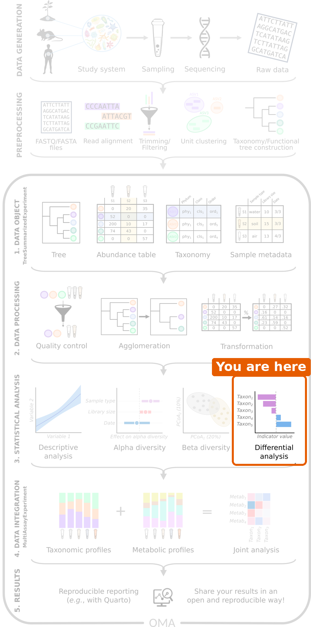
We now know that the gut microbiome of people with CRC differs from that of healthy people, both in diversity and in overall composition. The last question is: which bacteria differ?

Load packages and data

---

R

library(mia)
library(miaViz)
library(maaslin3)

For the tests, we use the daa package again. We used its daa::getWilcoxonTest() in the alpha diversity episode to test a colData column; here, its functions test the abundance of each taxon. As before, we write daa:: in front of its functions, for example daa::getTTest(), instead of loading the package with library().

R

tse <- readRDS(file.path("data", "tse_processed.rds"))

We set healthy as the first level of the disease factor. This makes it the reference group, so the results below compare CRC to healthy people:

R

tse$disease <- factor(tse$disease, levels = c("healthy", "CRC"))

Prepare the data

---

Abundances are very skewed: most values are small, and a few are very large. We therefore test the logarithm of the relative abundance. The logarithm of zero is not defined, so we first add a pseudocount of 1 to all counts. We do this in two steps with transformAssay(): first we calculate relative abundances from the counts plus one, and then we take their logarithm (base 10):

R

tse <- transformAssay(
    tse, assay.type = "counts", method = "relabundance",
    pseudocount = 1, name = "relabundance_pseudo"
)
tse <- transformAssay(
    tse, assay.type = "relabundance_pseudo", method = "log10",
    name = "log_relabundance"
)

On the log10 scale, a difference of 1 means ten times more.

Start with two taxa

---

Before testing hundreds of taxa, let’s look at two that we have already met: Prevotella copri and Faecalibacterium prausnitzii, a well-known butyrate producer. We make a TreeSE with only these two taxa (rows):

R

tse_sub <- tse[
    c("species-Prevotella_copri", "species-Faecalibacterium_prausnitzii"),
]

We plot their log relative abundance in each group:

R

plotBoxplot(
    tse_sub, assay.type = "log_relabundance", x = "disease",
    facet.by = "rownames"
)

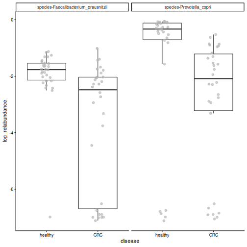
Both species tend to be more abundant in healthy people, but the groups overlap. The idea of differential abundance analysis (DAA) is to test whether differences like these are statistically significant, that is, larger than we would expect by chance.

A t-test

---

The simplest way to compare two groups is the t-test. The daa function daa::getTTest() runs one t-test per taxon. Its formula reads “the log_relabundance values are explained by disease”. var.equal = TRUE asks for the classic Student’s t-test:

R

res_t <- daa::getTTest(tse_sub, log_relabundance ~ disease, var.equal = TRUE)

OUTPUT

Registered S3 method overwritten by 'car':
  method           from
  na.action.merMod lme4

R

res_t

OUTPUT

# A tibble: 2 × 9
  rownames               .y.   group1 group2    n1    n2 statistic    df       p
* <chr>                  <chr> <chr>  <chr>  <int> <int>     <dbl> <dbl>   <dbl>
1 species-Faecalibacter… log_… healt… CRC       30    30      3.79    58 3.62e-4
2 species-Prevotella_co… log_… healt… CRC       30    30      2.35    58 2.21e-2

Each row is one taxon (rownames), and the column p holds its p-value.

Result: both species differ between the groups: P. copri (p = 0.022) and F. prausnitzii (p = 0.00036).

The t-test is a very elementary method, but it is a valid choice for microbiome data. A large comparison of DAA methods on 53 datasets found that simple methods, such as t-tests and linear models, give results that replicate better between datasets than many more complex methods (Pelto et al. 2025).

A linear model

---

A t-test can also be written as a linear model. The daa function daa::getLm() fits one linear model per taxon, with the same formula:

R

res_lm <- daa::getLm(tse_sub, log_relabundance ~ disease)
res_lm

OUTPUT

# A tibble: 2 × 5
  rownames                             variable   estimate  p_value  q_value
  <chr>                                <chr>         <dbl>    <dbl>    <dbl>
1 species-Prevotella_copri             diseaseCRC    -1.47 0.0221   0.0221
2 species-Faecalibacterium_prausnitzii diseaseCRC    -1.71 0.000362 0.000723

The p-values (p_value) are the same as those of the t-test: a t-test is a linear model with one two-group variable.

The advantage of the linear model is that we can add other variables, called covariates. In the beta diversity episode, we saw that the location also affects the microbiome. We add location to the formula, so that the effect of disease is tested while taking the location into account:

R

res_loc <- daa::getLm(tse_sub, log_relabundance ~ disease + location)
res_loc

OUTPUT

# A tibble: 4 × 5
  rownames                             variable       estimate  p_value  q_value
  <chr>                                <chr>             <dbl>    <dbl>    <dbl>
1 species-Prevotella_copri             diseaseCRC       -0.926 0.166    0.221
2 species-Prevotella_copri             locationKerala   -1.48  0.0420   0.0841
3 species-Faecalibacterium_prausnitzii diseaseCRC       -1.95  0.000204 0.000815
4 species-Faecalibacterium_prausnitzii locationKerala    0.634 0.234    0.234   

The results now have two rows per taxon: one for diseaseCRC and one for locationKerala.

Result: F. prausnitzii is still less abundant in CRC (p = 2e-04), but the disease effect of P. copri is no longer significant (p = 0.17). Most people from Kerala in our study have CRC, so part of the difference of P. copri may be due to the location rather than the disease.

Most DAA methods are based on this idea under the hood: they fit a model like this for every taxon, with the group of interest and the covariates.

Testing every taxon

---

So far we tested two taxa. In DAA, we usually test every taxon, and this brings a new problem.

Many tests, many false positives

With a p-value threshold of 0.05, we accept a 5 % chance of a false positive in each test. That is fine for one test, but with 100 taxa, about 5 of them would look significant by chance alone, even if nothing differed.

To avoid this, we correct for multiple testing. The corrected p-value is often called the q-value. The usual threshold is q < 0.05. The most common correction, the Benjamini–Hochberg method, controls the false discovery rate (FDR): if we report all taxa with q < 0.05, we expect at most 5 % of the reported taxa to be false positives.

Challenge

Challenge 1: False positives

You test 200 taxa with a p-value threshold of 0.05, but in reality none of them differ between the groups. About how many taxa will look significant anyway?

Show me the solution

About 200 × 0.05 = 10 taxa. This is why we correct for multiple testing.

Dedicated methods

---

The t-test and the linear model show what DAA does. Microbiome data has special features, though. The values are relative, so if one taxon increases, the shares of all others decrease. There are many zeros, as the box plot above shows: the samples at the bottom are those where the taxon was not detected at all. And the abundances are noisy: their spread changes with their level (the data is heteroscedastic).

Dedicated DAA methods extend the linear model to take these features into account. In this lesson we use MaAsLin 3. For each taxon, it fits two models:

• Abundance: when the taxon is present, is it more abundant in one group? This is a linear model on the log relative abundance, like the one above, but it uses only the samples where the taxon was detected.
• Prevalence: is the taxon present in more people of one group? This is a logistic regression on presence and absence. Much of the information in microbiome data is in the prevalence: whether a taxon is there at all is much less noisy than how much of it there is.

MaAsLin 3 also compares each taxon with the typical (median) taxon, because the data are relative, and it corrects the p-values for multiple testing. Many other methods exist, for example ANCOM-BC2 and ALDEx2, and they often give somewhat different results. See the Differential abundance chapter of OMA.

Run MaAsLin 3

---

As discussed in episode 5, we first remove rare taxa. They carry little information and add many tests:

R

tse <- subsetByPrevalent(
    tse, assay.type = "relabundance",
    detection = 0.001, prevalence = 0.1
)
nrow(tse)

OUTPUT

[1] 94

We give maaslin3() our TreeSE and a formula with disease and location. Unlike in daa::getLm(), the left side of the formula is empty: MaAsLin 3 puts each taxon there in turn. It uses the first table of the TreeSE (the counts) and transforms it itself. It writes its results to the folder given in output. The last three arguments switch off its own plots and most of its messages:

R

fit <- maaslin3(
    tse,
    formula = ~ disease + location,
    output = "maaslin3_output",
    plot_summary_plot = FALSE,
    plot_associations = FALSE,
    verbosity = "ERROR"
)

Differential abundance

---

The results of the abundance model are in fit$fit_data_abundance$results. The table has one row per taxon and variable, so we keep the rows for disease, and then the taxa with q < 0.05:

R

res <- fit$fit_data_abundance$results
res <- res[res$metadata == "disease", ]
sig <- res[res$qval_individual < 0.05 & !is.na(res$qval_individual), ]
sig[, c("feature", "coef", "qval_individual")]

OUTPUT

                                feature      coef qval_individual
1              species-Prevotella_copri -4.322978    3.137211e-06
3                      species-_rectale -3.499477    4.484035e-03
4  species-Faecalibacterium_prausnitzii -2.130628    4.484035e-03
5      species-Odoribacter_splanchnicus  4.312470    4.484035e-03
6        species-Prevotella_sp._AM42-24 -4.155679    4.484035e-03
7     species-Dialister_succinatiphilus -4.144146    8.424146e-03
8              species-Roseburia_faecis -4.396711    1.138791e-02
12 species-Firmicutes_bacterium_CAG-791  3.996070    2.555267e-02
13    species-Oscillibacter_sp._CAG-241  3.791330    2.976652e-02
16   species-Parabacteroides_distasonis  2.664330    4.367687e-02
17        species-Klebsiella_pneumoniae  6.313643    4.896360e-02

The most important columns are:

• feature: the taxon.
• coef: the effect size, the difference in log2 abundance. A positive value means the taxon is more abundant in CRC, a negative value that it is less abundant in CRC.
• stderr: the standard error of coef, that is, how uncertain it is.
• qval_individual: the q-value of this model, corrected for multiple testing.

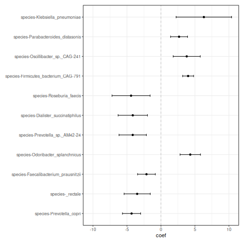
Result: 11 of the 94 species differ in abundance between people with CRC and healthy people: 5 are more abundant and 6 less abundant in CRC. The strongest result is Prevotella copri. In the linear model above, its difference was weaker once the location was taken into account. MaAsLin 3 looks only at the people who carry it, and among them, P. copri is much less abundant in CRC.

A forest plot shows the coefficient of each significant taxon, with an error bar for its uncertainty. The miaViz function plotForest() draws it from the results table:

R

plotForest(
    sig, effect.var = "coef", err.var = "stderr",
    id.var = "feature", pval.var = "qval_individual"
)

It is always a good idea to look at the data behind a result. We plot the relative abundances of the first four species of the list:

R

plotBoxplot(
    tse, assay.type = "relabundance", x = "disease",
    features = sig$feature[1:4], facet.by = "rownames"
)

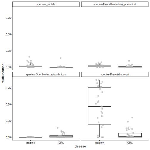
Result: the differences are clearly visible in the data, although the values of the two groups overlap.

Challenge

Challenge 2: Read the forest plot

1. Name two species that are more abundant in CRC, and two that are less abundant in CRC.
2. Faecalibacterium prausnitzii, Eubacterium rectale (shown as _rectale) and Roseburia faecis produce butyrate, a compound that helps to keep the gut lining healthy. In which group are they more abundant? Does this make sense?

Show me the solution

1. Species with a positive coefficient, such as Odoribacter splanchnicus, are more abundant in CRC. Species with a negative coefficient, such as Prevotella copri and Faecalibacterium prausnitzii, are less abundant in CRC.
2. They have negative coefficients: they are more abundant in healthy people. This makes sense: butyrate producers are often found to be depleted in CRC.

Challenge

Challenge 3: Without the location

1. Run MaAsLin 3 again with only disease in the formula. Save the results in a different folder, for example maaslin3_output_disease_only.
2. How many species differ in abundance (q < 0.05)?
3. How many of them were also significant in our first analysis?

Hint: intersect() gives the elements that two vectors share.

Show me the solution

R

fit2 <- maaslin3(
    tse,
    formula = ~ disease,
    output = "maaslin3_output_disease_only",
    plot_summary_plot = FALSE,
    plot_associations = FALSE,
    verbosity = "ERROR"
)
res2 <- fit2$fit_data_abundance$results
res2 <- res2[res2$metadata == "disease", ]
sig2 <- res2[res2$qval_individual < 0.05 & !is.na(res2$qval_individual), ]

nrow(sig2)

OUTPUT

[1] 12

R

length(intersect(sig$feature, sig2$feature))

OUTPUT

[1] 9

2. 12 species are significant.
3. 9 of them were also significant when the location was taken into account.

Some species are significant only when the location is ignored (3 here): their differences may be partly due to the location rather than the disease. Others are significant only when the location is in the formula (2 here): taking the location into account removes some of the noise, which makes a disease effect easier to detect. The choice of variables in the formula matters.

Differential prevalence

---

The results of the prevalence model are in fit$fit_data_prevalence$results. We keep the results for disease and the taxa with q < 0.05:

R

res_prevalence <- fit$fit_data_prevalence$results
res_prevalence <- res_prevalence[res_prevalence$metadata == "disease", ]
sig_prevalence <- res_prevalence[
    res_prevalence$qval_individual < 0.05 &
        !is.na(res_prevalence$qval_individual),
]
sig_prevalence[, c("feature", "coef", "qval_individual")]

OUTPUT

                                    feature      coef qval_individual
1             species-Bacteroides_eggerthii  3.815604     0.004484035
2              species-Bacteroides_fragilis  2.456524     0.004484035
4           species-Clostridium_sp._CAG-510  3.202124     0.004484035
5           species-Clostridium_sp._CAG-632  3.231433     0.004484035
6      species-Firmicutes_bacterium_CAG-238  3.788765     0.004484035
7            species-Flavonifractor_plautii  2.666713     0.004484035
8        species-Methanobrevibacter_smithii  3.145093     0.004484035
14          species-Bacteroides_sp._CAG-530  2.597764     0.011387908
15              species-Desulfovibrio_piger  2.572182     0.011387908
23     species-Bifidobacterium_adolescentis -2.035877     0.020664619
24                 species-Alistipes_shahii  2.028545     0.020883270
25            species-Klebsiella_pneumoniae -2.356969     0.021055323
26             species-Megasphaera_elsdenii -1.874297     0.021055323
29         species-Butyrivibrio_sp._CAG-318  2.258238     0.021186706
30           species-Roseburia_intestinalis -3.195097     0.021252854
35          species-Prevotella_sp._CAG-1092  2.031649     0.032098180
37 species-Intestinimonas_butyriciproducens  2.749107     0.032241998
38             species-Prevotella_stercorea  2.697288     0.036009251
41     species-Firmicutes_bacterium_CAG-110  1.956945     0.045155439
42            species-Mitsuokella_multacida -2.093394     0.048010635
3              species-Butyricimonas_virosa  2.922404     0.004484035
9                  species-Roseburia_faecis -2.894762     0.004484035
10  species-Ruthenibacterium_lactatiformans  2.758872     0.004484035
11              species-Veillonella_parvula  2.973239     0.004484035
12         species-Bacteroides_intestinalis  3.538988     0.006251335
13        species-Ligilactobacillus_ruminis -2.665089     0.011142771
17          species-Akkermansia_muciniphila  2.267651     0.014486316
18           species-Prevotella_sp._CAG-520  2.611054     0.016213310
19                         species-_rectale -2.209343     0.016605080

The prevalence model is a logistic regression: it models whether the taxon is present or absent. Its coef is the change in the log-odds of the taxon being present. The odds are the number of people who carry the taxon divided by the number who do not: 15 carriers and 15 non-carriers give odds of 1, 3 carriers and 27 non-carriers give odds of 1/9. You do not need to interpret the exact value. A positive value means that the taxon is found more often in CRC, and a negative value that it is found less often in CRC.

Result: 29 species differ in prevalence, of which 21 are found more often in CRC. Only 3 of them also differ in abundance. The prevalence model finds many results that the abundance model misses.

One of the prevalence results is Flavonifractor plautii. This is the bacterium that the authors of our study highlighted in the title of their paper. getPrevalence() gives the share of samples in which it is present, in each group:

R

getPrevalence(tse[, tse$disease == "CRC"], assay.type = "counts")["species-Flavonifractor_plautii"]

OUTPUT

species-Flavonifractor_plautii
                     0.7333333 

R

getPrevalence(tse[, tse$disease == "healthy"], assay.type = "counts")["species-Flavonifractor_plautii"]

OUTPUT

species-Flavonifractor_plautii
                     0.1333333 

R

plotBoxplot(
    tse, assay.type = "relabundance", x = "disease",
    features = "species-Flavonifractor_plautii"
)

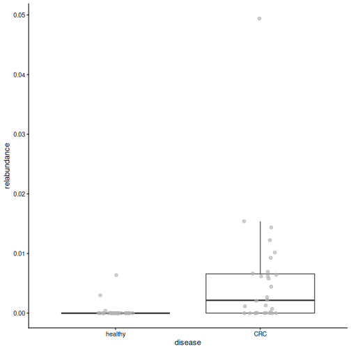
Result: F. plautii is present in 73 % of the CRC patients but in only 13 % of the healthy people. Its abundance is low in both groups: the clear difference is whether it is there.

Challenge

Challenge 4: Bacteroides fragilis

Some strains of Bacteroides fragilis produce a toxin that has been linked to CRC.

1. Find species-Bacteroides_fragilis in the prevalence results. What are its coef and qval_individual?
2. In what share of the CRC patients and of the healthy people is it present?
3. Does the sign of its coef agree with these shares?

Show me the solution

R

res_prevalence[
    res_prevalence$feature == "species-Bacteroides_fragilis",
    c("feature", "coef", "qval_individual")
]

OUTPUT

                       feature     coef qval_individual
2 species-Bacteroides_fragilis 2.456524     0.004484035

R

getPrevalence(tse[, tse$disease == "CRC"], assay.type = "counts")["species-Bacteroides_fragilis"]

OUTPUT

species-Bacteroides_fragilis
                         0.8 

R

getPrevalence(tse[, tse$disease == "healthy"], assay.type = "counts")["species-Bacteroides_fragilis"]

OUTPUT

species-Bacteroides_fragilis
                   0.2333333 

B. fragilis is present in more CRC patients than healthy people. Its coef is positive, which means “present more often in CRC”, so the sign agrees with the shares.

Challenge

Challenge 5 (optional): A famous CRC bacterium

Fusobacterium nucleatum is one of the bacteria most strongly linked to CRC in the literature, yet it is not in our results. Find out why.

Hint: load the unfiltered data from data/tse_processed.rds and calculate the prevalence of species-Fusobacterium_nucleatum with getPrevalence().

Show me the solution

R

tse_all <- readRDS(file.path("data", "tse_processed.rds"))
prevalence <- getPrevalence(tse_all, assay.type = "counts")
prevalence["species-Fusobacterium_nucleatum"]

OUTPUT

species-Fusobacterium_nucleatum
                     0.06666667 

F. nucleatum was detected in only 7 % of the people, so our prevalence filter (at least 10 % of samples) removed it before the analysis. Filtering always involves a trade-off: it makes the analysis more robust, but it can remove taxa that are rare but interesting.

Challenge

Challenge 6: How robust are the results? (30 minutes)

Our results depend on choices we made: the variables in the formula and the taxonomic rank. In this exercise, you test how robust they are.

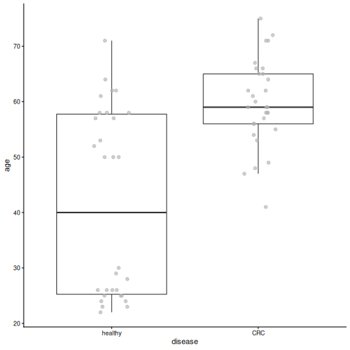
The CRC patients in our study are older than the healthy people (median age 59 vs 40 years), and age also affects the gut microbiome.

1. Plot age by disease with plotBoxplot(). Are there CRC patients under 40?
2. Run MaAsLin 3 with formula = ~ disease + location + age (output folder maaslin3_output_age). How many species differ in abundance by disease (q < 0.05)? Are any species associated with age itself?
3. Now repeat the analysis with ~ disease + location at the genus level (output folder maaslin3_output_genus). Load the full data again, agglomerate it with agglomerateByRank(), and prepare it as at the start of this episode. How many genera differ in abundance?
4. Is the genus Prevotella significant? Compare with the species-level result for Prevotella copri.
5. Write two or three sentences: which findings are robust to these choices, and which are not?

Show me the solution

1. Age by disease

R

plotBoxplot(tse, col.var = "age", x = "disease")

R

min(tse$age[tse$disease == "CRC"])

OUTPUT

[1] 41

All CRC patients are at least 41 years old, while many healthy people are younger.

2. MaAsLin 3 with age

R

fit_age <- maaslin3(
    tse,
    formula = ~ disease + location + age,
    output = "maaslin3_output_age",
    plot_summary_plot = FALSE,
    plot_associations = FALSE,
    verbosity = "ERROR"
)
res_age <- fit_age$fit_data_abundance$results
res_age <- res_age[res_age$qval_individual < 0.05 & !is.na(res_age$qval_individual), ]

sig_age_disease <- res_age[res_age$metadata == "disease", ]
sig_age_disease[, c("feature", "coef", "qval_individual")]

OUTPUT

                               feature      coef qval_individual
1             species-Prevotella_copri -4.270148    0.0002874643
3 species-Faecalibacterium_prausnitzii -2.512047    0.0441288103

R

sum(res_age$metadata == "age")

OUTPUT

[1] 0

With age in the formula, 2 species differ by disease (11 without age), and 0 species are associated with age. Age and disease are strongly linked in this study, so when both are in the model, it is hard to tell which of them explains a difference. The uncertainty of the disease effect grows and fewer results pass the threshold. To separate the effects of age and disease, we would need a study design in which the groups have similar ages (for example, age-matched controls).

3. and 4. Genus level

R

tse_genus <- readRDS(file.path("data", "tse_processed.rds"))
tse_genus <- agglomerateByRank(tse_genus, rank = "genus")
tse_genus$disease <- factor(tse_genus$disease, levels = c("healthy", "CRC"))
tse_genus <- transformAssay(
    tse_genus, assay.type = "counts", method = "relabundance"
)
tse_genus <- subsetByPrevalent(
    tse_genus, assay.type = "relabundance",
    detection = 0.001, prevalence = 0.1
)

fit_genus <- maaslin3(
    tse_genus,
    formula = ~ disease + location,
    output = "maaslin3_output_genus",
    plot_summary_plot = FALSE,
    plot_associations = FALSE,
    verbosity = "ERROR"
)
res_genus <- fit_genus$fit_data_abundance$results
res_genus <- res_genus[res_genus$metadata == "disease", ]
sum(res_genus$qval_individual < 0.05, na.rm = TRUE)

OUTPUT

[1] 7

R

res_genus[res_genus$feature == "Prevotella", c("feature", "coef", "qval_individual")]

OUTPUT

      feature      coef qval_individual
12 Prevotella -1.388461      0.05567889

At the genus level, 7 genera differ in abundance. The genus Prevotella is not significant (q = 0.056), although Prevotella copri was the strongest species-level result. The genus also contains other Prevotella species, and some of them, such as Prevotella sp. CAG-520, tend to be more abundant in CRC. Summing them with P. copri blurs the difference.

5. Conclusion

Results that hold across formulas and ranks are the most robust, for example the lower abundance of Prevotella copri and of the butyrate producer Faecalibacterium prausnitzii in CRC, which remain significant when age is added. Other results change when age is added or when we move to the genus level. The rank you analyse changes the question: “which species?” and “which genera?” are not the same question.

Key Points

• Differential abundance analysis tests whether the differences we see in plots are statistically significant.
• At its core, DAA is a simple test: a t-test is a linear model with one two-group variable, and a linear model can add covariates, such as the location. Most DAA methods are based on this under the hood.
• Testing many taxa produces false positives, so we use q-values that are corrected for multiple testing.
• Dedicated methods, such as MaAsLin 3, extend the linear model to take the specific nature of microbiome data into account: relative values, many zeros and noisy abundances.
• A taxon can differ in abundance, in prevalence (how often it is present), or both. MaAsLin 3 tests both.
• Look at the data behind the results, and treat significant taxa as candidates for further study.
• In our study, Prevotella copri and butyrate-producing species are less abundant in people with CRC, and Flavonifractor plautii is found much more often in CRC.