Machine learning: predicting an outcome

Overview

Questions

• How well can we predict an outcome, such as colorectal cancer, from the gut microbiome?
• Why do we split the data into training and test data?
• Which bacteria are the most important for the prediction?

Objectives

• Explain the terms feature, outcome, training data, test data, overfitting, cross-validation and AUC.
• Train a random forest model with mikropml to predict an outcome (here, the disease) from the abundance table.
• Evaluate a model with the cross-validation AUC and the test AUC, and explain why a single small test set is unreliable.
• Find the most important taxa of a model and compare them with the differential abundance results.

Where are we?

---

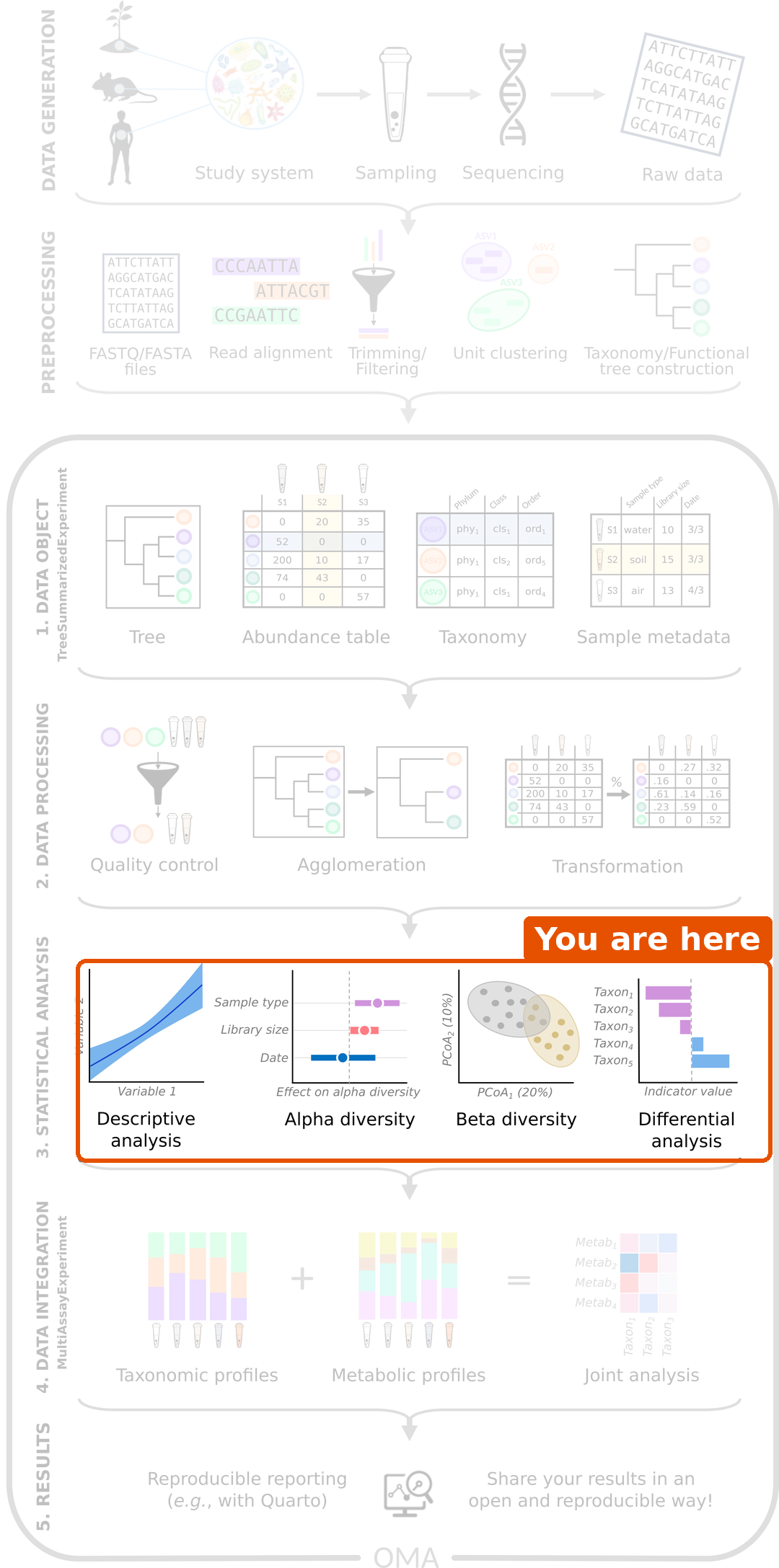
We are still in the statistical analysis step. In the beta diversity episode, the samples of people with CRC and healthy people largely separated in the ordination plots, and in the last episode we found which species differ between the groups. The next question is a practical one: if we only had a stool sample, how well could we tell whether the person has CRC? This is a prediction question, and machine learning is the usual tool for it. The outcome we predict can be anything we know about the samples, for example a disease, a treatment response or a diet; in our study, it is the disease.

Load packages and data

---

R

library(mia)
library(miaViz)
library(mikropml)
library(ggplot2)

R

tse <- readRDS(file.path("data", "tse_processed.rds"))

What is machine learning?

---

So far we have asked whether the groups differ. Machine learning asks whether we can predict the group of a new sample. A few terms:

Term	Meaning	In our data
Outcome	What we want to predict	disease: CRC or healthy
Features	What we use to predict it	The abundances of the taxa
Model	A set of rules learned from the data	A random forest
Hyperparameter	A setting of the model that is chosen before training, not learned from the data	mtry of the random forest (see below)
Training data	The samples the model learns from	80 % of the samples
Test data	Samples kept aside to check the model	The other 20 %

Why keep test data aside?

A flexible model can learn the training data by heart, including its random noise. It then looks perfect on the training data but fails on new samples. This is called overfitting. To get an honest estimate of how well the model works, we test it on samples that it has never seen.

The data is used like this:

1. The samples are split into training data (80 %) and test data (20 %).
2. On the training data, the model is tuned with cross-validation: the training data is split into 5 parts (folds), the model is trained on 4 and checked on the 5th, and this is repeated so that each fold is used for checking once. This gives the cross-validation (CV) performance. Tuning means that this is done for several values of the hyperparameters, and the values with the best CV performance are kept.
3. The final model is checked once on the test data. This gives the test performance.

Measuring performance: AUC

For each sample, the model gives a probability of CRC. The AUC (area under the ROC curve) measures how well these probabilities rank the samples:

• AUC = 1: every CRC sample gets a higher probability than every healthy sample.
• AUC = 0.5: no better than flipping a coin.

To turn the probabilities into a yes/no prediction, we need a cut-off, for example “CRC if the probability is above 0.5”. The ROC curve (receiver operating characteristic) shows what happens for every possible cut-off: how many of the CRC samples are found (the sensitivity), against how many of the healthy samples are wrongly called CRC (the false positive rate). The AUC is the area under this curve, so it does not depend on one chosen cut-off. Another common measure, the accuracy, is the share of samples predicted correctly at one cut-off.

Challenge

Challenge 1: Training and test data

A student trains a model on all 60 samples and then checks it on the same samples. The model gets an AUC of 1.0. Should the student be happy? Why or why not?

Show me the solution

No. The model was checked on the samples it learned from, so it may have memorized them (overfitting). The AUC of 1.0 says nothing about how the model works for new people. The model must be checked on samples it has not seen, such as a separate test set.

Prepare the data

---

We use the same taxa as in the differential abundance episode: the species that are found in at least 10 % of the samples.

R

tse_prevalent <- subsetByPrevalent(
    tse, assay.type = "relabundance",
    detection = 0.001, prevalence = 0.1
)

We use the raw counts as features: a random forest splits each feature into “high” and “low” values, so it does not need normally distributed or transformed data.

Train a random forest

---

A random forest is a collection of many decision trees. Each tree asks a series of questions such as “is the count of Prevotella copri above 10 000?” and ends with a prediction. The forest predicts by majority vote of its trees.

The most important hyperparameter of a random forest is mtry: the number of randomly chosen features that each question in a tree can pick from. A small mtry makes the trees more different from each other; a large mtry makes each tree stronger on its own. The best value depends on the data, so we let cross-validation choose it.

The mikropml function run_ml() works directly with a TreeSE. We give it the outcome as a column of colData (outcome_colname) and the features as an abundance table (assay.type). It then does all the steps from above: it splits the data into training and test data, tunes mtry with 5-fold cross-validation (kfold = 5, repeated cv_times = 5 times with different folds), and tests the final model. The seed makes the random split reproducible.

R

rf_results <- run_ml(
    tse_prevalent, method = "rf", outcome_colname = "disease",
    assay.type = "counts", kfold = 5, cv_times = 5, seed = 123
)

The mikropml functions get_hp_performance() and plot_hp_performance() show the CV AUC for each value of mtry that was tried:

R

hp <- get_hp_performance(rf_results$trained_model)
plot_hp_performance(hp$dat, mtry, AUC)

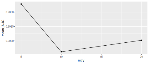
Result: all values of mtry give a similar CV AUC (note the narrow range of the y-axis), and run_ml() kept mtry = 5, the value with the highest CV AUC.

Evaluate the model

The performance is stored in rf_results$performance. The two most important columns are the cross-validation AUC of the chosen model and the test AUC:

R

rf_results$performance[, c("cv_metric_AUC", "AUC")]

OUTPUT

# A tibble: 1 × 2
  cv_metric_AUC   AUC
          <dbl> <dbl>
1         0.906     1

The mikropml function calc_model_sensspec() predicts the test data with the trained model and calculates the sensitivity and false positive rate for every cut-off. We plot them as a ROC curve. The dashed line is a model that guesses at random (AUC = 0.5):

R

sensspec <- calc_model_sensspec(
    rf_results$trained_model, rf_results$test_data, "disease"
)

OUTPUT

Using 'disease' as the outcome column.

R

ggplot(sensspec, aes(x = fpr, y = sensitivity)) +
    geom_step() +
    geom_abline(linetype = "dashed") +
    labs(x = "False positive rate", y = "Sensitivity")

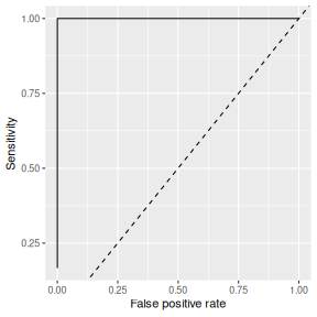
Result: the cross-validation AUC is 0.91, and the test AUC is 1. The gut microbiome predicts CRC very well in this study.

The CV AUC was used to choose mtry, so it is slightly optimistic. The test data was not used for any choice, so the test AUC is the honest estimate.

But the test set contains only 12 samples. With so few samples, a single lucky or unlucky split can change the test AUC a lot. Challenge 2 explores this.

Challenge

Challenge 2: How reliable is one test set?

The split into training and test data is random, and it is set by seed. Let’s see how much the test AUC depends on it.

1. Train the same random forest three more times, with seed = 4, seed = 5 and seed = 6. Store the results as rf_4, rf_5 and rf_6.
2. Combine the performance tables of the four models (rf_results and the three new ones) with rbind(), and plot them with the mikropml function plot_model_performance().
3. What are the smallest and largest test AUCs? What does this tell you about reporting the AUC of a single split?
4. Do the cross-validation AUCs vary as much? Why might that be?

Show me the solution

R

rf_4 <- run_ml(
    tse_prevalent, method = "rf", outcome_colname = "disease",
    assay.type = "counts", kfold = 5, cv_times = 5, seed = 4
)
rf_5 <- run_ml(
    tse_prevalent, method = "rf", outcome_colname = "disease",
    assay.type = "counts", kfold = 5, cv_times = 5, seed = 5
)
rf_6 <- run_ml(
    tse_prevalent, method = "rf", outcome_colname = "disease",
    assay.type = "counts", kfold = 5, cv_times = 5, seed = 6
)
performance <- rbind(
    rf_results$performance, rf_4$performance,
    rf_5$performance, rf_6$performance
)
performance[, c("seed", "cv_metric_AUC", "AUC")]

OUTPUT

# A tibble: 4 × 3
   seed cv_metric_AUC   AUC
  <dbl>         <dbl> <dbl>
1   123         0.906 1
2     4         0.958 0.833
3     5         0.919 1
4     6         0.978 0.722

R

plot_model_performance(performance)

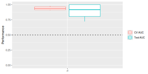
3. The test AUC ranges from 0.72 to 1. A single split of a small dataset can make a model look perfect or mediocre by chance. Report the performance over many splits (for example the median and range), not from one split. In practice, people use many more splits, for example 100; the mikropml documentation shows how to run them efficiently.
4. The cross-validation AUCs vary less (from 0.91 to 0.98), because each one is an average over 25 folds (5 folds, repeated 5 times) that together use all 48 training samples, while the test AUC comes from only 12 samples.

Which taxa matter most?

---

A model that predicts well is useful, but we also want to know which features it relies on. A random forest measures the importance of each feature: how much the questions about this feature help the trees to separate CRC from healthy samples, summed over all trees. mikropml trains the model with the caret package, so we get the importances with the caret function varImp(). It scales them from 0 (least important) to 100 (most important) and prints the most important features first:

R

importance <- caret::varImp(rf_results$trained_model)
importance

OUTPUT

rf variable importance

  only 20 most important variables shown (out of 94)

                                        Overall
species-Roseburia_faecis                 100.00
species-Prevotella_copri                  67.75
species-Odoribacter_splanchnicus          54.15
species-_rectale                          50.03
species-Bacteroides_fragilis              44.09
species-Flavonifractor_plautii            42.44
species-Parabacteroides_distasonis        42.16
species-Ruthenibacterium_lactatiformans   40.52
species-Ligilactobacillus_ruminis         39.92
species-Faecalibacterium_prausnitzii      36.55
species-Bacteroides_thetaiotaomicron      31.23
species-Bifidobacterium_adolescentis      30.58
species-Methanobrevibacter_smithii        29.87
species-Megasphaera_elsdenii              27.18
species-Alistipes_shahii                  24.88
species-Escherichia_coli                  23.32
species-Phocaeicola_vulgatus              20.12
species-Parabacteroides_merdae            19.54
species-Akkermansia_muciniphila           19.42
species-Bacteroides_intestinalis          18.99

caret also provides a ggplot() method for this object. We plot the ten most important species:

R

ggplot(importance, top = 10)

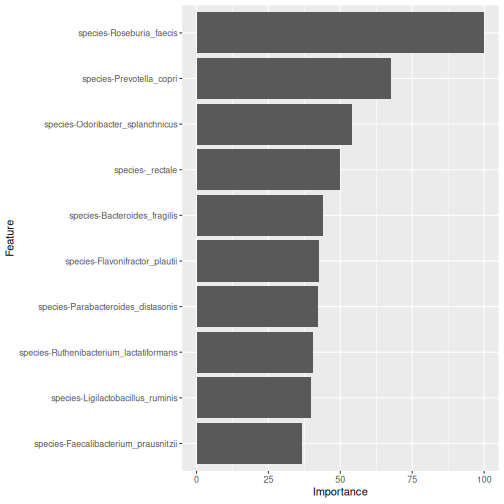
Result: the most important species is Roseburia faecis, followed by Prevotella copri and Odoribacter splanchnicus. Compare them with the differential abundance results of episode 8: many of the same species appear in both. Two very different methods point to the same bacteria.

Callout

Other importance measures

mikropml can also calculate permutation importance with run_ml(..., find_feature_importance = TRUE): it shuffles one feature at a time in the test data and measures how much the test AUC drops. With only 12 test samples, this estimate is very noisy, so we use the importance from the random forest itself. See the mikropml documentation.

Callout

Importance is not a difference

Feature importance tells us that a taxon helps the model to predict, but not in which direction: it does not say whether the taxon is higher in CRC or in healthy people. For that, look at the differential abundance results or plot the taxon by group with plotBoxplot().

Challenge

Challenge 3: A different model

mikropml supports other models too. A popular one is a regularized logistic regression, method = "glmnet". Unlike a random forest, it combines the features in a weighted sum, so it works best when the features are on a similar scale.

1. Prepare the relative abundances of tse_prevalent with the mikropml function preprocess_data() (outcome_colname = "disease", assay.type = "relabundance"). By default, it centres and scales each feature and removes features that carry no information. It adds the result to the TreeSE as a new table called preprocessed.
2. Train a glmnet model on the preprocessed table with the same settings as before.
3. Compare its cross-validation AUC with the random forest.

Show me the solution

R

tse_glm <- preprocess_data(
    tse_prevalent, outcome_colname = "disease", assay.type = "relabundance"
)
assayNames(tse_glm)

OUTPUT

[1] "counts"       "relabundance" "rclr"         "preprocessed"

R

glm_results <- run_ml(
    tse_glm, method = "glmnet", outcome_colname = "disease",
    assay.type = "preprocessed", kfold = 5, cv_times = 5, seed = 123
)
glm_results$performance[, c("cv_metric_AUC", "AUC")]

OUTPUT

# A tibble: 1 × 2
  cv_metric_AUC   AUC
          <dbl> <dbl>
1         0.884     1

The glmnet model has a cross-validation AUC of 0.88, compared with 0.91 for the random forest. Both predict CRC well. With only 60 samples, a small difference between the models could change with another split. glmnet is much faster, which matters for large datasets.

If preprocess_data() removes features, it stores the result as an alternative experiment instead, and you give run_ml() also altexp = "preprocessed". See the Machine learning chapter of OMA.

Challenge

Challenge 4: Genus level

Does the model work as well at the genus level?

1. Agglomerate the data to the genus level with agglomerateByRank().
2. Filter and train a random forest as above.
3. Compare the cross-validation AUC with the species-level model.

Show me the solution

R

tse_genus <- agglomerateByRank(tse, rank = "genus")
tse_genus <- transformAssay(
    tse_genus, assay.type = "counts", method = "relabundance"
)
tse_genus <- subsetByPrevalent(
    tse_genus, assay.type = "relabundance",
    detection = 0.001, prevalence = 0.1
)
genus_results <- run_ml(
    tse_genus, method = "rf", outcome_colname = "disease",
    assay.type = "counts", kfold = 5, cv_times = 5, seed = 123
)
genus_results$performance[, c("cv_metric_AUC", "AUC")]

OUTPUT

# A tibble: 1 × 2
  cv_metric_AUC   AUC
          <dbl> <dbl>
1         0.931 0.944

With 52 genera, the cross-validation AUC is 0.93, about the same as with species (0.91). The signal is strong at both levels.

Challenge

Challenge 5: Is it really the disease?

In our study, most people from Kerala have CRC (episode 4).

1. Make a table of location against disease.
2. Imagine a very simple “model”: predict CRC for everyone from Kerala and healthy for everyone from Bhopal. What share of the people would it classify correctly?
3. What does this mean for our microbiome model?

Show me the solution

R

location_table <- table(tse$location, tse$disease)
location_table

OUTPUT

         CRC healthy
  Bhopal  15      26
  Kerala  15       4

R

correct <- location_table["Kerala", "CRC"] + location_table["Bhopal", "healthy"]
correct / ncol(tse)

OUTPUT

[1] 0.6833333

2. The simple rule classifies 68 % of the people correctly, without looking at any bacteria.
3. Part of what the model learns could be the difference between Bhopal and Kerala rather than the disease. The microbiome model is much better than the location alone, but to be sure, it should be tested on new people, ideally from other places, or trained within one place only.

Callout

Before trusting a prediction model

• Small data. With 60 samples, performance estimates are uncertain. Report results over many splits.
• Independent validation. A model should be tested on an independent cohort, collected by other people in another place. Models often perform worse there.
• Confounding. If the groups differ in other ways (location, age, medication), the model may learn those differences instead of the disease.

See the Machine learning chapter of OMA.

Key Points

• Machine learning asks how well we can predict an outcome, such as a disease, from features, such as taxon abundances.
• Always evaluate a model on samples it has not seen: cross-validation on the training data and a separate test set.
• Hyperparameters, such as mtry of a random forest, are chosen by cross-validation on the training data only.
• mikropml works directly with a TreeSE: run_ml() trains, tunes and tests a model in one call, and preprocess_data() prepares the data when a model needs it. Random forests work on raw counts.
• The AUC measures how well the predictions separate the groups. With a small test set, it varies a lot between random splits.
• Feature importance shows which taxa the model relies on. In our study, many of them, such as Roseburia faecis, also differ in abundance.
• Confounders and small sample sizes can make a model look better than it is; independent validation is needed.