MultiAssayExperiment and the study data

Estimated time: 80 minutes

Overview

Questions

• What data do we analyse in this lesson?
• How do we store several data types of the same samples in R?
• How do we find out which samples have which data types?
• How do we prepare each data type for integration?

Objectives

• Describe the study design and the three data types of the HintikkaXO data.
• Describe the parts of a MultiAssayExperiment: the experiments, the sample information and the sample map, and how they differ from a TreeSummarizedExperiment.
• Access, explore and subset the experiments of a MultiAssayExperiment.
• Use an UpSet plot to see which samples have which data types, and keep only the samples that have all of them.
• Prepare each data type for integration, and explain why each data type gets its own transformation.

Where are we?

---

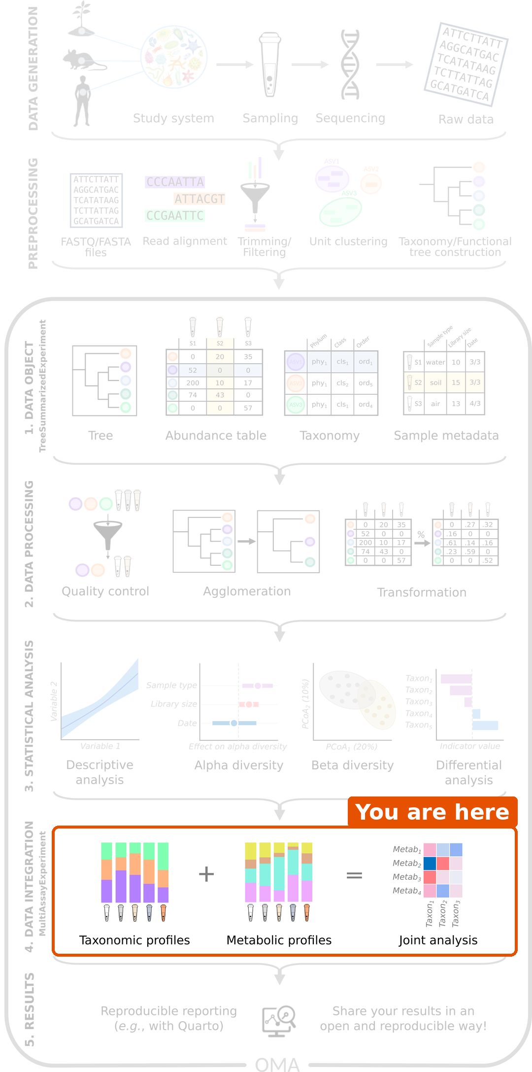
In a microbiome analysis, the first step is to store the data in one object, a TreeSummarizedExperiment (TreeSE). Integration starts the same way: we store all data types in one object, and prepare each of them for the analyses of the next episodes.

The study

---

We use data from a diet experiment in rats (Hintikka et al. 2021). Forty rats were fed one of four diets for several weeks:

	No supplement	XOS supplement
Low-fat diet	10 rats	10 rats
High-fat diet	10 rats	10 rats

A high-fat diet causes obesity and fatty liver. Xylo-oligosaccharides (XOS) are a prebiotic: a fibre that humans and rats cannot digest, but some gut bacteria can. The study asked whether XOS changes the gut microbiota and protects the rats from the harmful effects of the high-fat diet.

At the end of the experiment, three data types were measured for every rat:

• microbiota: the bacteria in the caecum (part of the gut), from 16S rRNA gene sequencing. The table contains read counts of taxa;
• metabolites: the concentrations of 38 known metabolites in the caecum, such as short-chain fatty acids, measured with nuclear magnetic resonance (NMR) spectroscopy;
• biomarkers: 39 lab measurements of host tissues, such as fat and microRNAs in the liver, and markers of inflammation in fat tissue. Each biomarker has its own unit.

The microbiota and the metabolites both come from the caecum content. The biomarkers come from other tissues of the same rat, such as the liver, fat tissue, muscle and blood. The three data types are truly different measurements, unlike taxa and pathways computed from the same reads (episode 1).

Note two things. The microbiota was measured with 16S amplicon sequencing, so the counts are real read counts and the taxa are reliable down to the genus. And the study is an experiment: the diet was set by the researchers, so all three data types may change with it. Keep this in mind. When two data types both change with the diet, they look related even if they do not affect each other directly.

The data comes with the mia package as the HintikkaXOData dataset, so there is nothing to download.

Load packages and data

---

R

library(mia)
library(miaViz)
library(MultiAssayExperiment)
library(ggplot2)

The data comes with mia. We load it with data() and give it a shorter name:

R

data("HintikkaXOData", package = "mia")
mae <- HintikkaXOData
mae

OUTPUT

A MultiAssayExperiment object of 3 listed
 experiments with user-defined names and respective classes.
 Containing an ExperimentList class object of length 3:
 [1] microbiota: TreeSummarizedExperiment with 12706 rows and 40 columns
 [2] metabolites: TreeSummarizedExperiment with 38 rows and 40 columns
 [3] biomarkers: TreeSummarizedExperiment with 39 rows and 40 columns
Functionality:
 experiments() - obtain the ExperimentList instance
 colData() - the primary/phenotype DataFrame
 sampleMap() - the sample coordination DataFrame
 `$`, `[`, `[[` - extract colData columns, subset, or experiment
 *Format() - convert into a long or wide DataFrame
 assays() - convert ExperimentList to a SimpleList of matrices
 exportClass() - save data to flat files

What is a MultiAssayExperiment?

---

A TreeSE holds one kind of feature (rows), such as taxa, measured from a set of samples (columns). Our study has three kinds of features: taxa, metabolites and biomarkers. To keep them together, Bioconductor has the MultiAssayExperiment (MAE) class.

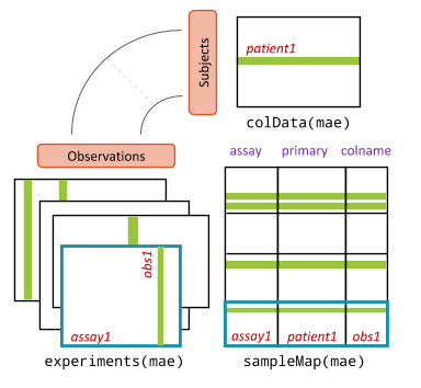
An MAE has three parts:

• experiments(): a list of experiments. Each experiment is one data type stored as its own object, here a TreeSE. The rows are the features and the columns are the samples, as before.
• colData(): one shared table of sample information, with one row per subject, here one row per rat.
• sampleMap(): a table that links each column of each experiment to a subject in colData(). Thanks to it, the MAE knows which columns belong to the same rat, even if they are named differently or in a different order.

Compared with a TreeSE:

	TreeSE	MAE
Data	Tables of the same features, assay()	Experiments with different features, experiments()
Pick one table	assay(tse, "counts")	mae[["microbiota"]] (a TreeSE)
Sample information	colData(tse), one row per column	colData(mae), one row per subject
Subset	tse[features, samples]	mae[features, subjects, experiments]

The printout above shows that our MAE has three experiments, all with 40 columns: microbiota with 12706 rows (taxa), metabolites with 38 rows and biomarkers with 39 rows.

Look inside the MultiAssayExperiment

---

names() gives the names of the experiments, and [[ picks one of them. The result is an ordinary TreeSE, and all the usual TreeSE functions work on it:

R

names(mae)

OUTPUT

[1] "microbiota"  "metabolites" "biomarkers" 

R

mae[["metabolites"]]

OUTPUT

class: TreeSummarizedExperiment
dim: 38 40
metadata(0):
assays(1): nmr
rownames(38): Butyrate Acetate ... Malonate 1,3-dihydroxyacetone
rowData names(0):
colnames(40): C1 C2 ... C39 C40
colData names(0):
reducedDimNames(0):
mainExpName: NULL
altExpNames(0):
rowLinks: NULL
rowTree: NULL
colLinks: NULL
colTree: NULL

R

assayNames(mae[["metabolites"]])

OUTPUT

[1] "nmr"

R

assay(mae[["metabolites"]], "nmr")[1:5, 1:5]

OUTPUT

                C1     C2      C3      C4      C5
Butyrate    0.9441 0.9605  2.2940  0.8100  0.6623
Acetate     9.0399 8.8941 18.4768 14.9939 16.7815
Propionate  2.0856 2.2319  3.6512  3.4386  4.0731
Valerate    0.3554 0.3351  0.6565  0.4298  0.4812
Isovalerate 0.0998 0.1116  0.1312  0.1084  0.0858

The shared sample information is in colData(), and $ accesses one of its columns, as with a TreeSE:

R

colData(mae)

OUTPUT

DataFrame with 40 rows and 6 columns
         Sample      Rat        Site          Diet      Fat       XOS
    <character> <factor> <character>      <factor> <factor> <numeric>
C1           C1        1       Cecum      High-fat     High         0
C2           C2        2       Cecum      High-fat     High         0
C3           C3        3       Cecum      High-fat     High         0
C4           C4        4       Cecum      High-fat     High         0
C5           C5        5       Cecum      High-fat     High         0
...         ...      ...         ...           ...      ...       ...
C36         C36       36       Cecum Low-fat + XOS      Low         1
C37         C37       37       Cecum Low-fat + XOS      Low         1
C38         C38       38       Cecum Low-fat + XOS      Low         1
C39         C39       39       Cecum Low-fat + XOS      Low         1
C40         C40       40       Cecum Low-fat + XOS      Low         1

R

table(mae$Fat, mae$XOS)

OUTPUT

        0  1
  Low  10 10
  High 10 10

Each of the four diets has 10 rats. The column XOS is a number (0 or 1). We turn it into a factor with clear labels, which will make the plots easier to read:

R

mae$XOS <- factor(mae$XOS, levels = c(0, 1), labels = c("control", "XOS"))
table(mae$Diet, mae$XOS)

OUTPUT

                 control XOS
  High-fat            10   0
  High-fat + XOS       0  10
  Low-fat             10   0
  Low-fat + XOS        0  10

Finally, sampleMap() shows how the columns of the experiments are linked to the rats:

R

sampleMap(mae)

OUTPUT

DataFrame with 120 rows and 3 columns
         assay     primary     colname
      <factor> <character> <character>
1   microbiota          C1          C1
2   microbiota          C2          C2
3   microbiota          C3          C3
4   microbiota          C4          C4
5   microbiota          C5          C5
...        ...         ...         ...
116 biomarkers         C36         C36
117 biomarkers         C37         C37
118 biomarkers         C38         C38
119 biomarkers         C39         C39
120 biomarkers         C40         C40

There is one row for each column of each experiment: 3 experiments × 40 samples = 120 rows. The column assay is the experiment, primary is the subject (the rat, a row of colData(mae)), and colname is the name of the column in the experiment. For rat C1, there is one column in each experiment:

R

sampleMap(mae)[sampleMap(mae)$primary == "C1", ]

OUTPUT

DataFrame with 3 rows and 3 columns
        assay     primary     colname
     <factor> <character> <character>
1 microbiota           C1          C1
2 metabolites          C1          C1
3 biomarkers           C1          C1

In our data, primary and colname are the same, because each rat has one sample per data type with the same name. They differ when the names differ, for example C1_16S and C1_NMR, or when a rat has several samples in one experiment, for example C1_week0 and C1_week8 before and after the diet. Both columns then have the primary C1, and they share the sample information of rat C1.

Experiments with the sample information

The experiments inside the MAE have no sample information of their own: it is stored once, in colData(mae).

R

colData(mae[["microbiota"]])

OUTPUT

DataFrame with 40 rows and 0 columns

When we need the sample information in an experiment, for example to colour a plot by diet, getWithColData() returns the experiment with the matching rows of colData(mae) added:

R

tse <- getWithColData(mae, "microbiota")

WARNING

Warning: 'experiments' dropped; see 'drops()'

R

colData(tse)

OUTPUT

DataFrame with 40 rows and 6 columns
         Sample      Rat        Site          Diet      Fat      XOS
    <character> <factor> <character>      <factor> <factor> <factor>
C1           C1        1       Cecum      High-fat     High  control
C2           C2        2       Cecum      High-fat     High  control
C3           C3        3       Cecum      High-fat     High  control
C4           C4        4       Cecum      High-fat     High  control
C5           C5        5       Cecum      High-fat     High  control
...         ...      ...         ...           ...      ...      ...
C36         C36       36       Cecum Low-fat + XOS      Low      XOS
C37         C37       37       Cecum Low-fat + XOS      Low      XOS
C38         C38       38       Cecum Low-fat + XOS      Low      XOS
C39         C39       39       Cecum Low-fat + XOS      Low      XOS
C40         C40       40       Cecum Low-fat + XOS      Low      XOS

getWithColData() warns that 'experiments' dropped: it takes one experiment out of the MAE and leaves the others behind. The warning is harmless.

Challenge

Challenge 1: Explore the biomarkers

1. Which tables (assays) does the biomarkers experiment contain?
2. List the names of the first ten biomarkers.
3. How many values are missing (NA) in the biomarkers? Hint: is.na() and sum().
4. Which biomarker has the most missing values?

Show me the solution

R

assayNames(mae[["biomarkers"]])

OUTPUT

[1] "signals"

R

head(rownames(mae[["biomarkers"]]), 10)

OUTPUT

 [1] "Triglycerides_liver" "CLSs_epi"            "Mononucl_epi"
 [4] "miR21_liver"         "miR122_liver"        "miR192_liver"
 [7] "miR221_liver"        "CD45_Epi"            "CD45_Mese"
[10] "IL1b_mese"          

R

sum(is.na(assay(mae[["biomarkers"]], "signals")))

OUTPUT

[1] 95

R

na_per_biomarker <- rowSums(is.na(assay(mae[["biomarkers"]], "signals")))
head(sort(na_per_biomarker, decreasing = TRUE))

OUTPUT

     HAD_epi     AST_mese     ALT_mese miR122_liver miR192_liver miR221_liver
          15           11           10            5            5            5 

1. One assay, signals.
2. The names describe the measurement and the tissue, for example Triglycerides_liver (fat in the liver) or CD45_Epi (immune cells in the fat tissue around the testes, the epididymal fat).
3. 95 values are missing.
4. HAD_epi, with 15 missing values out of 40.

Which samples have which data types?

---

In our study, every rat has all three data types. In real studies, this is often not the case: a sample fails in sequencing, or there was not enough material to measure the metabolites. The MAE handles this without problems, because the sampleMap() records which rats each experiment has.

To see how this looks, we make a copy of the data in which the biomarkers are missing for the last 10 rats:

R

mae_incomplete <- mae
mae_incomplete[["biomarkers"]] <- mae_incomplete[["biomarkers"]][, 1:30]

OUTPUT

harmonizing input:
  removing 10 sampleMap rows with 'colname' not in colnames of experiments

R

mae_incomplete

OUTPUT

A MultiAssayExperiment object of 3 listed
 experiments with user-defined names and respective classes.
 Containing an ExperimentList class object of length 3:
 [1] microbiota: TreeSummarizedExperiment with 12706 rows and 40 columns
 [2] metabolites: TreeSummarizedExperiment with 38 rows and 40 columns
 [3] biomarkers: TreeSummarizedExperiment with 39 rows and 30 columns
Functionality:
 experiments() - obtain the ExperimentList instance
 colData() - the primary/phenotype DataFrame
 sampleMap() - the sample coordination DataFrame
 `$`, `[`, `[[` - extract colData columns, subset, or experiment
 *Format() - convert into a long or wide DataFrame
 assays() - convert ExperimentList to a SimpleList of matrices
 exportClass() - save data to flat files

An UpSet plot shows how many samples have each combination of data types. The function upsetSamples() draws it:

R

upsetSamples(mae_incomplete)

OUTPUT

Install the required package(s) with:

  BiocManager::install("UpSetR")

ERROR

Error:
! The calling function requires missing package dependencies:
  "UpSetR"

Each column of the bottom panel is a combination of experiments (the connected dots), and the bar above it shows the number of samples with that combination.

Result: 30 rats have all three data types, and 10 rats have only the microbiota and the metabolites.

Many integration methods need the same samples in every experiment. intersectColumns() keeps only the samples that are in all experiments:

R

intersectColumns(mae_incomplete)

OUTPUT

A MultiAssayExperiment object of 3 listed
 experiments with user-defined names and respective classes.
 Containing an ExperimentList class object of length 3:
 [1] microbiota: TreeSummarizedExperiment with 12706 rows and 30 columns
 [2] metabolites: TreeSummarizedExperiment with 38 rows and 30 columns
 [3] biomarkers: TreeSummarizedExperiment with 39 rows and 30 columns
Functionality:
 experiments() - obtain the ExperimentList instance
 colData() - the primary/phenotype DataFrame
 sampleMap() - the sample coordination DataFrame
 `$`, `[`, `[[` - extract colData columns, subset, or experiment
 *Format() - convert into a long or wide DataFrame
 assays() - convert ExperimentList to a SimpleList of matrices
 exportClass() - save data to flat files

Subset the MultiAssayExperiment

---

An MAE is subset with [ , ] like a TreeSE. The columns are the samples, and the subset is applied to all experiments at once. Here we keep only the rats on the high-fat diet:

R

mae_highfat <- mae[, mae$Fat == "High"]
mae_highfat

OUTPUT

A MultiAssayExperiment object of 3 listed
 experiments with user-defined names and respective classes.
 Containing an ExperimentList class object of length 3:
 [1] microbiota: TreeSummarizedExperiment with 12706 rows and 20 columns
 [2] metabolites: TreeSummarizedExperiment with 38 rows and 20 columns
 [3] biomarkers: TreeSummarizedExperiment with 39 rows and 20 columns
Functionality:
 experiments() - obtain the ExperimentList instance
 colData() - the primary/phenotype DataFrame
 sampleMap() - the sample coordination DataFrame
 `$`, `[`, `[[` - extract colData columns, subset, or experiment
 *Format() - convert into a long or wide DataFrame
 assays() - convert ExperimentList to a SimpleList of matrices
 exportClass() - save data to flat files

Result: each experiment now has 20 samples. The data types and the sample information stay in sync.

To keep only some experiments, we use the third index:

R

mae[, , c("microbiota", "metabolites")]

OUTPUT

A MultiAssayExperiment object of 2 listed
 experiments with user-defined names and respective classes.
 Containing an ExperimentList class object of length 2:
 [1] microbiota: TreeSummarizedExperiment with 12706 rows and 40 columns
 [2] metabolites: TreeSummarizedExperiment with 38 rows and 40 columns
Functionality:
 experiments() - obtain the ExperimentList instance
 colData() - the primary/phenotype DataFrame
 sampleMap() - the sample coordination DataFrame
 `$`, `[`, `[[` - extract colData columns, subset, or experiment
 *Format() - convert into a long or wide DataFrame
 assays() - convert ExperimentList to a SimpleList of matrices
 exportClass() - save data to flat files

To keep only some features, subsetByRow() takes a list with the rows to keep in each experiment. Here we keep three short-chain fatty acids and all biomarkers:

R

subsetByRow(mae, list(metabolites = c("Butyrate", "Acetate", "Propionate"),
                      biomarkers = rownames(mae[["biomarkers"]])))

OUTPUT

A MultiAssayExperiment object of 3 listed
 experiments with user-defined names and respective classes.
 Containing an ExperimentList class object of length 3:
 [1] microbiota: TreeSummarizedExperiment with 12706 rows and 40 columns
 [2] metabolites: TreeSummarizedExperiment with 3 rows and 40 columns
 [3] biomarkers: TreeSummarizedExperiment with 39 rows and 40 columns
Functionality:
 experiments() - obtain the ExperimentList instance
 colData() - the primary/phenotype DataFrame
 sampleMap() - the sample coordination DataFrame
 `$`, `[`, `[[` - extract colData columns, subset, or experiment
 *Format() - convert into a long or wide DataFrame
 assays() - convert ExperimentList to a SimpleList of matrices
 exportClass() - save data to flat files

Experiments that are not in the list lose all their rows.

Prepare the data

---

Each data type needs its own preparation before integration. The methods of the next episodes expect values that are roughly normally distributed. Rare features, which are zero in most samples, add noise rather than information. The data types are measured in different ways (episode 1), so each needs its own transformation:

Experiment	Values	Preparation
microbiota	Read counts; compositional	Agglomerate, filter rare genera, rclr
metabolites	Concentrations; skewed, some below the detection limit	Replace NA with 0, log10
biomarkers	Different units and scales, some NA	Keep as they are

Microbiota

The microbiota experiment has 12706 taxa, many of them rare. We prepare it as in a single-table analysis: we agglomerate the taxa to genera, keep the prevalent genera and transform the counts. First, we look at the taxonomy:

R

tse <- mae[["microbiota"]]
head(rowData(tse), 3)

OUTPUT

DataFrame with 3 rows and 7 columns
                                  Phylum                  Class
                             <character>            <character>
GAYR01026362.62.2014 D_1__Proteobacteria D_2__Alphaproteobact..
CVJT01000011.50.2173     D_1__Firmicutes           D_2__Bacilli
KF625183.1.1786      D_1__Proteobacteria D_2__Gammaproteobact..
                                      Order                 Family
                                <character>            <character>
GAYR01026362.62.2014     D_3__Rickettsiales      D_4__Mitochondria
CVJT01000011.50.2173        D_3__Bacillales D_4__Staphylococcaceae
KF625183.1.1786      D_3__Enterobacteriales D_4__Enterobacteriac..
                                      Genus                Species
                                <character>            <character>
GAYR01026362.62.2014 D_5__Solanum melonge.. D_6__Solanum melonge..
CVJT01000011.50.2173    D_5__Staphylococcus D_6__Staphylococcus ..
KF625183.1.1786             D_5__Klebsiella D_6__Klebsiella oxyt..
                                      OTU
                              <character>
GAYR01026362.62.2014 GAYR01026362.62.2014
CVJT01000011.50.2173 CVJT01000011.50.2173
KF625183.1.1786           KF625183.1.1786

Each name has a prefix that tells its rank, such as D_4__ for a family and D_5__ for a genus. The prefixes come from the SILVA taxonomy database, and many datasets have them. They do not change the analysis, so we keep them.

Now we agglomerate to genera, add relative abundances, keep the genera that are found in at least 20 % of the rats with a relative abundance above 0.1 %, and add an rclr table. The rclr transformation removes the effect of the sequencing depth and makes the values closer to normally distributed:

R

tse <- agglomerateByRank(tse, rank = "Genus")
tse <- transformAssay(tse, assay.type = "counts", method = "relabundance")
tse <- subsetByPrevalent(tse, assay.type = "relabundance",
                         detection = 0.001, prevalence = 0.2)
tse <- transformAssay(tse, assay.type = "counts", method = "rclr")
tse

OUTPUT

class: TreeSummarizedExperiment
dim: 57 40
metadata(1): agglomerated_by_rank
assays(3): counts relabundance rclr
rownames(57): Ambiguous_taxa_3 D_5__[Eubacterium] coprostanoligenes
  group ... D_5__uncultured_3 D_5__uncultured_4
rowData names(7): Phylum Class ... Species OTU
colnames(40): C1 C2 ... C39 C40
colData names(0):
reducedDimNames(0):
mainExpName: NULL
altExpNames(0):
rowLinks: NULL
rowTree: NULL
colLinks: NULL
colTree: NULL

Some genera are called uncultured: they are known only from their DNA and have no proper name. Their names are not unique, so mia adds a number, such as D_5__uncultured_2.

We put the prepared TreeSE back into the MAE:

R

mae[["microbiota"]] <- tse

Result: the microbiota now has 57 prevalent genera, with the assays counts, relabundance and rclr.

Metabolites

The metabolite concentrations have some missing values:

R

sum(is.na(assay(mae[["metabolites"]], "nmr")))

OUTPUT

[1] 27

They are in only 8 of the 38 metabolites. We treat them as values below the detection limit of NMR: the metabolite was there in too small amounts to be measured. So we replace them with 0. If the values were missing because a measurement failed, this would be wrong.

The metabolites are absolute concentrations, not compositional counts, so we do not use rclr. Concentrations are skewed (a few very high values), so we add a log10 table. The logarithm of 0 is not defined, so pseudocount = TRUE first adds half of the smallest concentration above 0 to all values:

R

met <- mae[["metabolites"]]
assay(met, "nmr")[is.na(assay(met, "nmr"))] <- 0
met <- transformAssay(met, assay.type = "nmr", method = "log10",
                      pseudocount = TRUE)

OUTPUT

A pseudocount of 0.00045 was applied.

R

mae[["metabolites"]] <- met
assayNames(mae[["metabolites"]])

OUTPUT

[1] "nmr"   "log10"

Biomarkers

The biomarkers are a mix of lab measurements, each with its own unit and scale, and some have missing values (challenge 1). One transformation does not fit all of them, so we keep them as they are. Where a method needs values on the same scale, such as MOFA in episode 4, we standardize each biomarker. MOFA also handles the missing values itself; for other methods, we drop the biomarkers with missing values.

Challenge

Challenge 2: Do the diets differ?

Before integrating the data types, it is good to look at each of them alone.

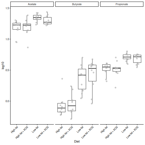
1. Draw box plots of the log10 concentrations of butyrate, acetate and propionate by Diet. Hint: use getWithColData() to get the metabolites with the sample information. Then use plotBoxplot() with features = ..., x = "Diet" and facet.by = "rownames".
2. Make a PCA of the microbiota from its rclr table, and colour the rats by Fat and shape them by XOS. Hint: runPCA() from scater and plotReducedDim().
3. Which factor, the fat or the XOS, has a larger effect on the metabolites and on the microbiota?

Show me the solution

R

met <- getWithColData(mae, "metabolites")
plotBoxplot(met, assay.type = "log10", x = "Diet",
            features = c("Butyrate", "Acetate", "Propionate"),
            facet.by = "rownames") +
    theme(axis.text.x = element_text(angle = 45, hjust = 1))

R

library(scater)
tse <- getWithColData(mae, "microbiota")
tse <- runPCA(tse, assay.type = "rclr", name = "PCA", ncomponents = 3)
plotReducedDim(tse, "PCA", colour_by = "Fat", shape_by = "XOS")

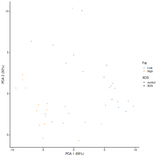
The fat content of the diet has by far the larger effect. The high-fat rats have less butyrate, acetate and propionate than the low-fat rats, and the high-fat and low-fat rats are separated along the first axis of the PCA. The effect of XOS is small in both data types. Keep this in mind: in the next episodes, the strongest shared patterns will be about fat.

Keep the object

---

We use the prepared mae object in all the next episodes, so keep your R session open. If you restart R, run the code of this episode again: the data comes with mia, so this takes only a few seconds.

Callout

Your own data

To build an MAE from your own data, first create one TreeSE (or SummarizedExperiment) per data type, then combine them:

R

mae <- MultiAssayExperiment(
    experiments = ExperimentList(microbiota = tse_taxa,
                                 metabolites = tse_metabolites),
    colData = sample_info
)

If the columns of the experiments are named differently from the rows of sample_info, also give a sampleMap. See the OMA chapter on data containers and the MultiAssayExperiment vignette.

Key Points

• The HintikkaXO data has three data types from 40 rats: microbiota, metabolites and host biomarkers. The rats were fed a high-fat or a low-fat diet, with or without the prebiotic XOS.
• A MultiAssayExperiment holds several experiments (here three TreeSEs), one shared table of sample information (colData()) and a sampleMap() that links them.
• [[ picks one experiment, and $ accesses the sample information. getWithColData() returns an experiment together with the sample information.
• upsetSamples() shows which samples have which data types, and intersectColumns() keeps the samples that have all of them.
• Subsetting by samples keeps all experiments in sync. subsetByRow() subsets the features of each experiment.
• sampleMap() links each column (colname) of each experiment to a subject (primary) in colData().
• Each data type needs its own preparation: we agglomerate, filter and rclr-transform the compositional microbiota, replace values below the detection limit and log-transform the metabolites, and keep the biomarkers as they are.