Exploratory methods

Estimated time: 95 minutes

Overview

Questions

• Are the gut bacteria and the metabolites related?
• Which metabolites are related to the microbiota as a whole?
• Which genera go together with which metabolites?

Objectives

• Explain the idea of a Mantel test, and use it to test whether two data types are related overall.
• Find the features of one data type that relate to the whole other data type with MiRKAT.
• Calculate, plot and interpret pairwise associations between genera and metabolites.
• Explain why a shared factor, such as the diet, can create associations between data types, and check this by repeating an analysis within each diet group.

Where are we?

---

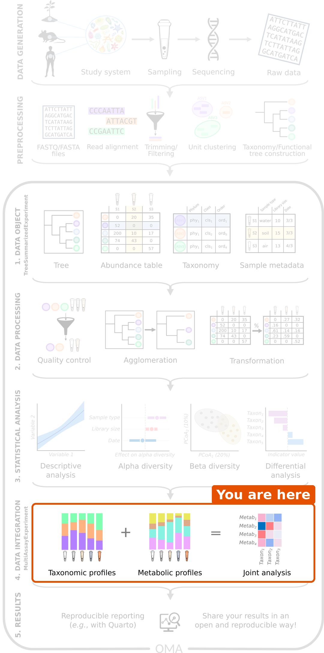
In the previous episode, we stored and prepared the three data types in a MultiAssayExperiment. Now we start to integrate them. The exploratory methods of this episode go from the big picture to the details:

Step	Question	Method
1	Are the two data types related overall?	Mantel test
2	Which metabolites relate to the whole microbiota?	MiRKAT
3	Which genera go together with which metabolites?	Pairwise association

We focus on two data types, the microbiota and the metabolites.

Load packages

---

The methods come from the multiomics package of the OMA framework. It is not yet in Bioconductor; the setup instructions install it from GitHub.

R

library(mia)
library(miaViz)
library(MultiAssayExperiment)
library(multiomics)
library(ggplot2)

We continue with the mae object that we prepared in episode 2:

R

mae

OUTPUT

A MultiAssayExperiment object of 3 listed
 experiments with user-defined names and respective classes.
 Containing an ExperimentList class object of length 3:
 [1] microbiota: TreeSummarizedExperiment with 57 rows and 40 columns
 [2] metabolites: TreeSummarizedExperiment with 38 rows and 40 columns
 [3] biomarkers: TreeSummarizedExperiment with 39 rows and 40 columns
Functionality:
 experiments() - obtain the ExperimentList instance
 colData() - the primary/phenotype DataFrame
 sampleMap() - the sample coordination DataFrame
 `$`, `[`, `[[` - extract colData columns, subset, or experiment
 *Format() - convert into a long or wide DataFrame
 assays() - convert ExperimentList to a SimpleList of matrices
 exportClass() - save data to flat files

All methods below take the same arguments:

• experiments: which two experiments to compare, here c(1, 2) for microbiota and metabolites;
• assay.types: which table to use from each experiment, here rclr for the microbiota and log10 for the metabolites.

The methods may warn that 'experiments' dropped. They take the two experiments out of the MAE, and the warning is harmless.

1. Are the data types related? The Mantel test

---

The Mantel test (Mantel 1967) compares two dissimilarity matrices. For each pair of rats, we calculate one dissimilarity based on the microbiota and one based on the metabolites. If rats that are similar in their microbiota are also similar in their metabolites, the two dissimilarities are correlated.

We use the Euclidean distance for both. On the rclr values of the microbiota, this is the robust Aitchison distance.

Is the correlation larger than we would expect by chance? Like PERMANOVA, the Mantel test answers this with permutations: it shuffles the rats of one table many times, recalculates the correlation each time, and checks how often the shuffled correlation is as large as the real one. This is why we set a seed.

R

set.seed(123)
mantel <- getMantel(mae, experiments = c(1, 2),
                    assay.types = c("rclr", "log10"),
                    dist.methods = c("euclidean", "euclidean"))
mantel

OUTPUT

Mantel statistic based on Kendall's rank correlation tau

Call:
mantel(xdis = x[[1L]], ydis = x[[2L]], method = method, permutations = npermutations,      strata = strata, na.rm = na.rm, parallel = parallel)

Mantel statistic r: 0.1138
      Significance: 0.011

Upper quantiles of permutations (null model):
   90%    95%  97.5%    99%
0.0607 0.0780 0.0947 0.1111
Permutation: free
Number of permutations: 999

The Mantel statistic r is the correlation between the two dissimilarity matrices (by default, Kendall’s rank correlation), and Significance is its permutation p-value. The correlations of the shuffled data are stored in mantel$perm. A histogram shows where the real correlation (red line) lies among them:

R

hist(mantel$perm, breaks = 30, main = "Mantel test",
     xlab = "Correlation of shuffled data")
abline(v = mantel$statistic, col = "red", lwd = 2)

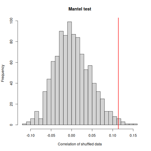
Result: the microbiota and the metabolites are related (r = 0.11, p = 0.011): rats with similar gut bacteria tend to have similar metabolites in the gut. Few shuffled correlations are as large as the real one. Still, the correlation is weak, so each data type also carries much information that the other does not.

Challenge

Challenge 1: Is it only the diet?

Both the microbiota and the metabolites differ between the high-fat and the low-fat rats (episode 2). Could the Mantel result be caused only by the diet, and not by a direct link between bacteria and metabolites?

1. Subset mae to the rats on the high-fat diet.
2. Repeat the Mantel test on this subset.
3. Is the association stronger or weaker than with all rats? What does this tell you?

Show me the solution

R

mae_highfat <- mae[, mae$Fat == "High"]
set.seed(123)
mantel_highfat <- getMantel(mae_highfat, experiments = c(1, 2),
                            assay.types = c("rclr", "log10"),
                            dist.methods = c("euclidean", "euclidean"))
mantel_highfat$statistic

OUTPUT

[1] 0.09161793

R

mantel_highfat$signif

OUTPUT

[1] 0.167

Within the high-fat rats, r = 0.09 and p = 0.17. The association is weaker than with all rats.

When two data types both depend on a third factor, such as the diet, they are correlated even if they do not affect each other. Part of the association over all rats comes from the diet. Comparing rats within one diet group removes this part. With only 20 rats, the test also has less power.

2. Which metabolites relate to the microbiota? MiRKAT

---

The Mantel test gives one number for the whole tables. MiRKAT (the microbiome regression-based kernel association test; Zhao et al. 2015) goes one step further: it tests, for each metabolite, whether the metabolite is related to the microbiota as a whole.

The idea: MiRKAT turns the microbiota distances into a kernel, a matrix of similarities between the rats. It then asks whether rats with a similar microbiota also have similar values of the metabolite. This is like a regression of the metabolite on all genera at once, without estimating one coefficient per genus, which would be impossible with 57 genera and 40 rats.

R

mirkat <- getMiRKAT(mae, experiments = c(1, 2),
                    assay.types = c("rclr", "log10"),
                    dist.methods = "euclidean")
head(mirkat)

OUTPUT

            p_values_euclidean krv_euclidean r2_euclidean
Butyrate          9.669747e-07  8.333548e-06  0.194115404
Acetate           1.649362e-02  2.716656e-06  0.020628585
Propionate        6.032696e-03  3.392296e-06  0.032165309
Valerate          8.499944e-02  1.607873e-06  0.007226096
Isovalerate       1.237908e-02  2.910570e-06  0.023678608
Isobutyrate       2.037613e-01  1.029617e-06  0.002963135

There is one row per metabolite. p_values_euclidean is the p-value, and r2_euclidean estimates the share of the metabolite’s variation that is explained by the microbiota, like the R2 of a regression. (krv_euclidean is another measure of association that we do not use.) We correct the p-values for multiple testing:

R

mirkat$qval <- p.adjust(mirkat$p_values_euclidean, method = "fdr")
sum(mirkat$qval < 0.05)

OUTPUT

[1] 7

We plot the 15 metabolites with the highest R2. The highest values are at the bottom:

R

mirkat_top <- mirkat[order(mirkat$r2_euclidean, decreasing = TRUE)[1:15], ]
plot(mirkat_top, column = "r2_euclidean")

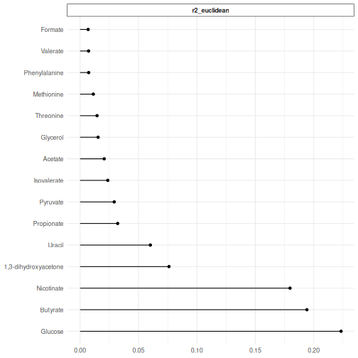
Result: 7 of the 38 metabolites are significantly related to the microbiota (q < 0.05): Glucose, Butyrate, Nicotinate, 1,3-dihydroxyacetone, Uracil, Propionate, Pyruvate. The microbiota explains up to 22 % of the variation of a single metabolite.

Butyrate, propionate and acetate are short-chain fatty acids that gut bacteria produce when they ferment fibre, so it makes sense that they are related to the microbiota.

3. Which genera go with which metabolites? Pairwise association

---

Now we look at pairs of features: for every genus and every metabolite, we calculate a correlation across the rats (by default Kendall’s tau).

With 57 genera and 38 metabolites, the heatmap would be hard to read. We keep the 20 most abundant genera with subsetByRow(), which we met in episode 2:

R

top_genera <- getTop(mae[["microbiota"]], top = 20, assay.type = "relabundance")
mae_top <- subsetByRow(mae, list(microbiota = top_genera,
                                 metabolites = rownames(mae[["metabolites"]])))

assoc <- getPairwiseAssociation(mae_top, experiments = c(1, 2),
                                assay.types = c("rclr", "log10"))
head(assoc)

OUTPUT

                      feature1 feature2       value
1         D_5__Parabacteroides Butyrate  0.34358974
2               D_5__Alistipes Butyrate -0.18461538
3  D_5__uncultured bacterium_1 Butyrate  0.46923077
4 D_5__Ruminococcaceae UCG-014 Butyrate  0.07179487
5             D_5__Bacteroides Butyrate  0.06923077
6             D_5__Akkermansia Butyrate -0.40512821

Each row is one pair of features (feature1 is the genus, feature2 the metabolite) with its association (value), from −1 to 1. The plot() function draws a heatmap, with the genera and metabolites ordered so that similar patterns are next to each other:

R

plot(assoc) +
    theme(axis.text.x = element_text(angle = 45, hjust = 1))

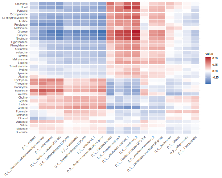
Result: the strongest association is between D_5__uncultured_2 and Glucose (0.54). Groups of genera show the same pattern across the metabolites, often because they respond to the diet in the same way.

Callout

Correlation is not causation

A strong association between a genus and a metabolite can mean that the genus produces or uses the metabolite. But it can also mean that both depend on something else, such as the diet (challenge 1). Genera that tend to occur together also share their associations. Treat associations as hypotheses to follow up.

Challenge

Challenge 2: Read the heatmap

1. Find butyrate in the heatmap. Which genera are positively associated with it, and which negatively?
2. Make the heatmap again with Spearman’s correlation (method = "spearman"). Does the picture change?

Show me the solution

R

assoc_spearman <- getPairwiseAssociation(mae_top, experiments = c(1, 2),
                                         assay.types = c("rclr", "log10"),
                                         method = "spearman")
plot(assoc_spearman) +
    theme(axis.text.x = element_text(angle = 45, hjust = 1))

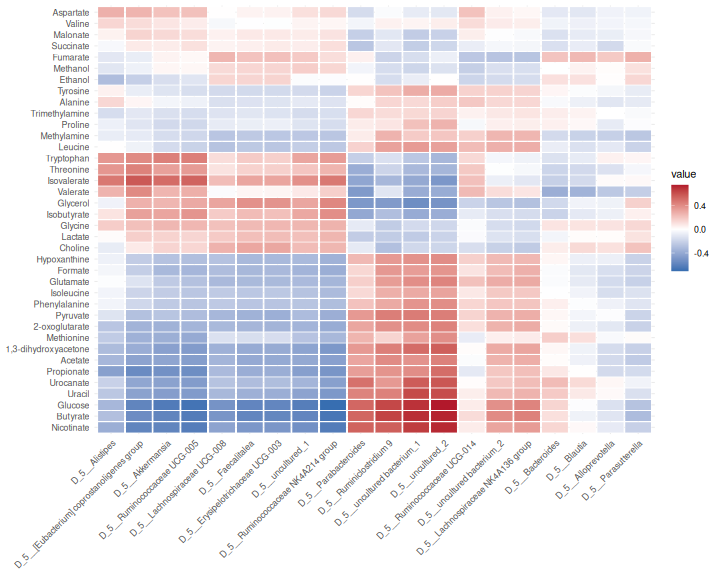
1. With Kendall’s tau, the genera most positively associated with butyrate are D_5__uncultured_2, D_5__uncultured bacterium_1, D_5__Ruminiclostridium 9, and the most negatively associated are D_5__Ruminococcaceae NK4A214 group, D_5__Ruminococcaceae UCG-005, D_5__uncultured_1.

2. Spearman’s correlations are larger in size than Kendall’s tau, because the two measure the association on different scales. The pattern (which pairs are positive and which negative) is very similar.

Challenge

Challenge 3 (about 30 minutes): Who goes with butyrate?

Butyrate is a short-chain fatty acid that feeds the cells of the gut wall, and it was among the metabolites most strongly related to the microbiota (MiRKAT). Which genera go together with butyrate?

1. Create an MAE that contains all genera and only butyrate. Hint: subsetByRow().
2. Calculate the association between butyrate and every genus with getPairwiseAssociation() and Spearman’s correlation.
3. Which five genera have the strongest positive association with butyrate, and which five the strongest negative association?
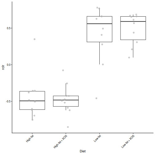
4. Draw a box plot of the rclr abundance of the most positively associated genus by Diet. Compare it with the box plot of butyrate from challenge 2 of episode 2. Hint: getWithColData() and plotBoxplot().
5. Calculate the association between butyrate and the same genus again, but within each fat group. Hint: the argument group.by = "Fat". Is the association still there, or does it come mainly from the difference between the diet groups?

Show me the solution

R

mae_butyrate <- subsetByRow(mae, list(microbiota = rownames(mae[["microbiota"]]),
                                      metabolites = "Butyrate"))
assoc_butyrate <- getPairwiseAssociation(mae_butyrate, experiments = c(1, 2),
                                         assay.types = c("rclr", "log10"),
                                         method = "spearman")
assoc_butyrate <- assoc_butyrate[order(assoc_butyrate$value, decreasing = TRUE), ]

head(assoc_butyrate[, c("feature1", "value")], 5)

OUTPUT

                      feature1     value
55           D_5__uncultured_2 0.7262664
52 D_5__uncultured bacterium_1 0.7033771
10           D_5__Anaerostipes 0.6675422
32          D_5__Oscillibacter 0.6604128
33          D_5__Papillibacter 0.6495310

R

tail(assoc_butyrate[, c("feature1", "value")], 5)

OUTPUT

                             feature1      value
42 D_5__Ruminococcaceae NK4A214 group -0.6606004
24             D_5__Lachnoclostridium -0.6637899
49                       D_5__UBA1819 -0.6889306
29                D_5__Marvinbryantia -0.7215760
27                 D_5__Lactobacillus -0.7309568

R

genus <- as.character(assoc_butyrate$feature1[1])
tse <- getWithColData(mae, "microbiota")
plotBoxplot(tse, assay.type = "rclr", x = "Diet", features = genus) +
    theme(axis.text.x = element_text(angle = 45, hjust = 1))

R

mae_genus <- subsetByRow(mae, list(microbiota = genus,
                                   metabolites = "Butyrate"))
assoc_groups <- getPairwiseAssociation(mae_genus, experiments = c(1, 2),
                                       assay.types = c("rclr", "log10"),
                                       method = "spearman", group.by = "Fat")
assoc_groups

OUTPUT

           feature1 feature2      value strata
1 D_5__uncultured_2 Butyrate 0.02406015   High
2 D_5__uncultured_2 Butyrate 0.41654135    Low

D_5__uncultured_2 has the strongest positive association with butyrate (0.73). Like butyrate, it is higher in the low-fat rats than in the high-fat rats. Within the groups, the association is much weaker: 0.02 in the high-fat rats and 0.42 in the low-fat rats. Much of the association over all rats comes from the difference between the diet groups.

This is the lesson of challenge 1 again: an association over all samples can be driven by a shared factor. To find links that hold within a diet, we can analyse the groups separately (group.by), or remove the effect of the diet before calculating the associations (the argument formula, see ?getPairwiseAssociation).

Callout

Other exploratory methods

The multiomics package also has getJointRDA() (redundancy analysis of one data type constrained by the other) and getLASSO() (a sparse regression of each feature of one data type on the other). The Bioconductor package anansi tests only the pairs that make biological sense, for example a bacterium and the metabolites that its enzymes can produce. See the OMA chapters on multi-omics and cross-association.

References

---

• Mantel N. (1967) The detection of disease clustering and a generalized regression approach. Cancer Research 27: 209–220.
• Zhao N. et al. (2015) Testing in microbiome-profiling studies with MiRKAT, the microbiome regression-based kernel association test. American Journal of Human Genetics 96: 797–807.

Key Points

• Exploratory integration goes from the big picture to the details: global association, feature vs data type, and feature vs feature.
• getMantel() tests whether two data types are related overall; getMiRKAT() finds the features of one data type that relate to the other as a whole.
• getPairwiseAssociation() calculates the association of every pair of features; subsetByRow() keeps the result small enough to plot.
• The Mantel test and MiRKAT are permutation or kernel tests: they compare similarities between samples instead of single features.
• A shared factor, such as the diet, creates associations between data types. Check associations within each group (group.by). Associations are hypotheses, not proof that a bacterium produces a metabolite.