19 Cross-association
Cross-association analysis is a straightforward approach that can reveal strength and type of associations between data sets. For instance, we can analyze if higher presence of a specific taxon relates to higher levels of a biomolecule. Correlation analyses within dataset were already discussed in Chapter 17.
As an example dataset, we use the data from the Hintikka et al. (2021) publication: Xylo-Oligosaccharides in prevention of hepatic steatosis and adipose tissue inflammation: associating taxonomic and metabolomic patterns in fecal microbiota with biclustering. In this study, mice were fed either with a high-fat or a low-fat diet, and with or without prebiotics, for the purpose of studying whether prebiotics attenuate the negative impact of a high-fat diet on health.
This example data can be loaded from the mia package. The data is already in MAE format which is tailored for multi-assay analyses (see Chapter 3). The dataset includes three different experiments: microbial abundance data, metabolite concentrations, and data about different biomarkers. If you like to construct the same data object from the original files instead, here you can find help for importing data into an SE object.
# Load the data
data(HintikkaXOData, package = "mia")
mae <- HintikkaXOData
# Available alternative experiments
experiments(mae)
## ExperimentList class object of length 3:
## [1] microbiota: TreeSummarizedExperiment with 12706 rows and 40 columns
## [2] metabolites: TreeSummarizedExperiment with 38 rows and 40 columns
## [3] biomarkers: TreeSummarizedExperiment with 39 rows and 40 columns# Microbiome data
getWithColData(mae, "microbiota")
## class: TreeSummarizedExperiment
## dim: 12706 40
## metadata(0):
## assays(1): counts
## rownames(12706): GAYR01026362.62.2014 CVJT01000011.50.2173 ...
## JRJTB:03787:02429 JRJTB:03787:02478
## rowData names(7): Phylum Class ... Species OTU
## colnames(40): C1 C2 ... C39 C40
## colData names(6): Sample Rat ... Fat XOS
## reducedDimNames(0):
## mainExpName: NULL
## altExpNames(0):
## rowLinks: NULL
## rowTree: NULL
## colLinks: NULL
## colTree: NULL# Metabolite data
getWithColData(mae, "metabolites")
## class: TreeSummarizedExperiment
## dim: 38 40
## metadata(0):
## assays(1): nmr
## rownames(38): Butyrate Acetate ... Malonate 1,3-dihydroxyacetone
## rowData names(0):
## colnames(40): C1 C2 ... C39 C40
## colData names(6): Sample Rat ... Fat XOS
## reducedDimNames(0):
## mainExpName: NULL
## altExpNames(0):
## rowLinks: NULL
## rowTree: NULL
## colLinks: NULL
## colTree: NULL# Biomarker data
getWithColData(mae, "biomarkers")
## class: TreeSummarizedExperiment
## dim: 39 40
## metadata(0):
## assays(1): signals
## rownames(39): Triglycerides_liver CLSs_epi ... NPY_serum
## Glycogen_liver
## rowData names(0):
## colnames(40): C1 C2 ... C39 C40
## colData names(6): Sample Rat ... Fat XOS
## reducedDimNames(0):
## mainExpName: NULL
## altExpNames(0):
## rowLinks: NULL
## rowTree: NULL
## colLinks: NULL
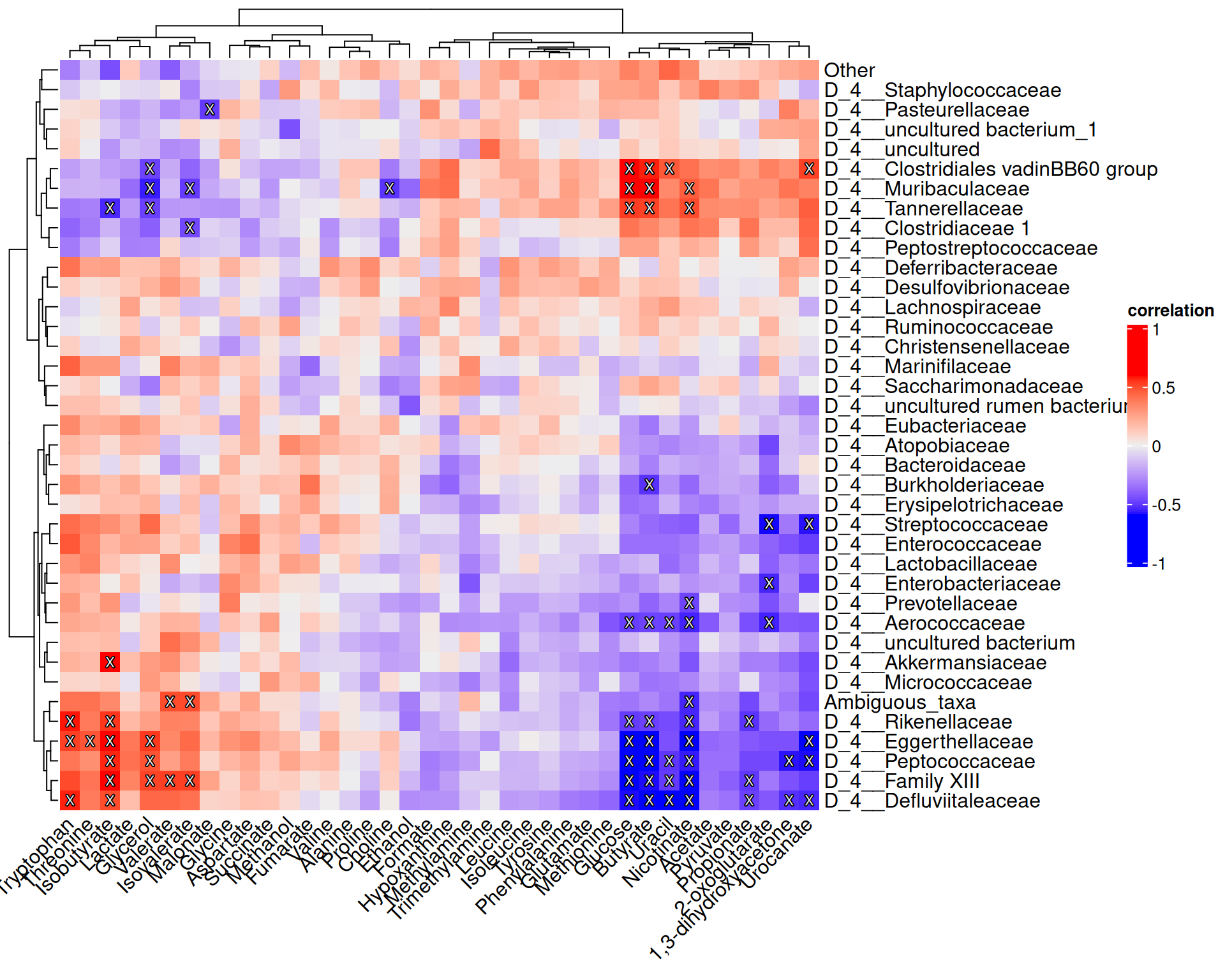
## colTree: NULLNext we can perform a cross-association analysis. Let us analyze if individual bacteria genera are correlated with concentrations of individual metabolites. This helps to answer the following question: “If bacterium X is present, is the concentration of metabolite Y lower or higher”?
# Agglomerate microbiome data at family level
mae[[1]] <- agglomerateByPrevalence(mae[[1]], rank = "Family", na.rm = TRUE)
# Does log10 transform for microbiome data
mae[[1]] <- transformAssay(mae[[1]], method = "log10", pseudocount = TRUE)

# Cross correlates data sets
res <- getCrossAssociation(
    mae,
    experiment1 = 1,
    experiment2 = 2,
    assay.type1 = "log10",
    assay.type2 = "nmr",
    method = "spearman",
    test.signif = TRUE,
    p.adj.threshold = NULL,
    cor.threshold = NULL,
    # Remove when mia is fixed
    mode = "matrix",
    sort = TRUE,
    show.warnings = FALSE
)
Next, we create a heatmap depicting all cross-correlations between bacterial genera and metabolite concentrations.
library(ComplexHeatmap)
library(shadowtext)

# Function for marking significant correlations with "X"
add_signif <- function(j, i, x, y, width, height, fill) {
    # If the p-value is under threshold
    if (!is.na(res$p_adj[i, j]) & res$p_adj[i, j] < 0.05) {
        # Print "X"
        grid.shadowtext(
            sprintf("%s", "X"), x, y,
            gp = gpar(fontsize = 8, col = "#f5f5f5")
        )
    }
}

# Create a heatmap
p <- Heatmap(res$cor,
    # Print values to cells
    cell_fun = add_signif,
    heatmap_legend_param = list(
        title = "correlation", legend_height = unit(5, "cm")
    ),
    column_names_rot = 45
)
p