6 Taxonomic information
Taxonomic information is a key part of analyzing microbiome data, and without it, any type of data analysis probably would not make much sense. However, the degree of detail of taxonomic information differs depending on the dataset and annotation data used.
Therefore, the mia package expects a loose assembly of taxonomic information and assumes certain key aspects:
- Taxonomic information is given as character vectors or factors in the
rowDataof a SummarizedExperiment object. - The columns containing the taxonomic information must be named
domain,kingdom,phylum,class,order,family,genus,speciesor with a capital first letter. - The columns must be given in the order shown above.
- A column can be omitted, but the order must remain.
In this chapter, we will refer to the co-abundant groups as CAGs, which are clusters of taxonomic features that co-vary across samples.
6.1 Assigning taxonomic information
There are a number of methods to assign taxonomic information. We like to give a short introduction about the methods available without ranking one over the other. This has to be your choice based on the result for the individual dataset.
6.1.1 DADA2
The dada2 package (Callahan et al. 2016) implements the assignTaxonomy() function, which takes as input the ASV sequences associated with each row of data and a training dataset. For more information visit the dada2 homepage.
6.1.2 DECIPHER
The DECIPHER package (Wright 2020) implements the IDTAXA algorithm to assign either taxonomic information or function information. For mia, only the first option is of interest for now and more information can be found on the DECIPHER website.
6.2 Functions to access taxonomic information
6.2.1 Check taxonomy ranks in data
checkTaxonomy() checks whether the taxonomic information is usable for mia.
checkTaxonomy(tse)
##  [1] TRUE
Since the rowData can contain other data, taxonomyRanks() will return the columns that mia assumes to contain the taxonomic information.
taxonomyRanks(tse)
##  [1] "Kingdom" "Phylum"  "Class"   "Order"   "Family"  "Genus"   "Species"
This can then be used to subset the rowData to columns as needed.
rowData(tse)[, taxonomyRanks(tse)]
##  DataFrame with 19216 rows and 7 columns
##             Kingdom        Phylum        Class        Order        Family
##         <character>   <character>  <character>  <character>   <character>
##  549322     Archaea Crenarchaeota Thermoprotei           NA            NA
##  522457     Archaea Crenarchaeota Thermoprotei           NA            NA
##  951        Archaea Crenarchaeota Thermoprotei Sulfolobales Sulfolobaceae
##  244423     Archaea Crenarchaeota        Sd-NA           NA            NA
##  586076     Archaea Crenarchaeota        Sd-NA           NA            NA
##  ...            ...           ...          ...          ...           ...
##  278222    Bacteria           SR1           NA           NA            NA
##  463590    Bacteria           SR1           NA           NA            NA
##  535321    Bacteria           SR1           NA           NA            NA
##  200359    Bacteria           SR1           NA           NA            NA
##  271582    Bacteria           SR1           NA           NA            NA
##               Genus                Species
##         <character>            <character>
##  549322          NA                     NA
##  522457          NA                     NA
##  951     Sulfolobus Sulfolobusacidocalda..
##  244423          NA                     NA
##  586076          NA                     NA
##  ...            ...                    ...
##  278222          NA                     NA
##  463590          NA                     NA
##  535321          NA                     NA
##  200359          NA                     NA
##  271582          NA                     NA
taxonomyRankEmpty() checks for empty values in the given rank and returns a logical vector of length(x).
all(!taxonomyRankEmpty(tse, rank = "Kingdom"))
##  [1] TRUE
table(taxonomyRankEmpty(tse, rank = "Genus"))
##
##  FALSE  TRUE
##   8008 11208
table(taxonomyRankEmpty(tse, rank = "Species"))
##
##  FALSE  TRUE
##   1413 17803
6.2.2 Get taxonomy labels
getTaxonomyLabels() is a multi-purpose function, which turns taxonomic information into a character vector of length(x)
getTaxonomyLabels(tse) |> head()
##  [1] "Class:Thermoprotei"               "Class:Thermoprotei_1"
##  [3] "Species:Sulfolobusacidocaldarius" "Class:Sd-NA"
##  [5] "Class:Sd-NA_1"                    "Class:Sd-NA_2"
By default, this will use the lowest non-empty information to construct a string with the following scheme level:value. If all levels are the same, this part is omitted, but can be added by setting with.rank = TRUE.
phylum <- !is.na(rowData(tse)$Phylum) &
    vapply(data.frame(apply(
        rowData(tse)[, taxonomyRanks(tse)[3:7]], 1L, is.na
    )), all, logical(1))
getTaxonomyLabels(tse[phylum, ]) |> head()
##  [1] "Crenarchaeota"    "Crenarchaeota_1"  "Crenarchaeota_2"
##  [4] "Actinobacteria"   "Actinobacteria_1" "Spirochaetes"
getTaxonomyLabels(tse[phylum, ], with.rank = TRUE) |> head()
##  [1] "Phylum:Crenarchaeota"    "Phylum:Crenarchaeota_1"
##  [3] "Phylum:Crenarchaeota_2"  "Phylum:Actinobacteria"
##  [5] "Phylum:Actinobacteria_1" "Phylum:Spirochaetes"
By default the return value of getTaxonomyLabels() contains only unique elements by passing it through make.unique. This step can be omitted by setting make.unique = FALSE.
getTaxonomyLabels(tse[phylum, ], with.rank = TRUE, make.unique = FALSE) |> head()
##  [1] "Phylum:Crenarchaeota"  "Phylum:Crenarchaeota"  "Phylum:Crenarchaeota"
##  [4] "Phylum:Actinobacteria" "Phylum:Actinobacteria" "Phylum:Spirochaetes"
To apply the loop resolving function resolveLoop() from the TreeSummarizedExperiment package (Huang 2020) within getTaxonomyLabels(), set resolve.loops = TRUE.
6.2.3 Get information on specific features
The function getUnique() gives a list of unique features for the specified taxonomic rank.
With mapTaxonomy(), you can search information on certain taxonomic features from the taxonomy table. For instance, we can check all the features that matches with “Escherichia”.
mapTaxonomy(tse, taxa = "Escherichia")
##  $Escherichia
##  DataFrame with 1 row and 7 columns
##             Kingdom         Phylum               Class             Order
##         <character>    <character>         <character>       <character>
##  249227    Bacteria Proteobacteria Gammaproteobacteria Enterobacteriales
##                     Family       Genus     Species
##                <character> <character> <character>
##  249227 Enterobacteriaceae Escherichia          NA
6.3 Prune taxonomy tree
Subsetting is explained in detail in Chapter 9. However, if you’ve already subsetted your data, you may have noticed that the taxonomy tree does not automatically update when using the [] operators. Although the linkages between rows and tree nodes remain correct, the tree retains its original, complex structure. You may be wondering how to update the tree to reflect the newly simplified data.
mia package functions subsetBy* and agglomerateBy* (see Chapter 10) include an update.tree parameter to handle this adjustment. However, when using [], tree pruning must be done as an additional step.
Let’s start by selecting 5 arbitrary rows.
tse_sub <- tse[1:5, ]
tse_sub
##  class: TreeSummarizedExperiment
##  dim: 5 26
##  metadata(0):
##  assays(1): counts
##  rownames(5): 549322 522457 951 244423 586076
##  rowData names(7): Kingdom Phylum ... Genus Species
##  colnames(26): CL3 CC1 ... Even2 Even3
##  colData names(7): X.SampleID Primer ... SampleType Description
##  reducedDimNames(0):
##  mainExpName: NULL
##  altExpNames(0):
##  rowLinks: a LinkDataFrame (5 rows)
##  rowTree: 1 phylo tree(s) (19216 leaves)
##  colLinks: NULL
##  colTree: NULL
Even though we have only 5 rows, the tree still retains its original number of tips. To align the tree with the subsetted data, we can use the TreeSummarizedExperiment´s subsetByLeaf() function, which allows us to select specific tips from the tree, effectively pruning it to match the current subset of data.
tse_sub <- subsetByLeaf(tse_sub, rowLeaf = rownames(tse_sub))
tse_sub
##  class: TreeSummarizedExperiment
##  dim: 5 26
##  metadata(0):
##  assays(1): counts
##  rownames(5): 549322 522457 951 244423 586076
##  rowData names(7): Kingdom Phylum ... Genus Species
##  colnames(26): CL3 CC1 ... Even2 Even3
##  colData names(7): X.SampleID Primer ... SampleType Description
##  reducedDimNames(0):
##  mainExpName: NULL
##  altExpNames(0):
##  rowLinks: a LinkDataFrame (5 rows)
##  rowTree: 1 phylo tree(s) (5 leaves)
##  colLinks: NULL
##  colTree: NULL
Now, we can see that the taxonomy tree has a simpler structure, including only the selected leaves.
6.4 Generate a hierarchy tree on the fly
A hierarchy tree shows mapping between the taxonomic levels in taxonomic rank table (included in rowData), rather than the detailed phylogenetic relations. Usually, a phylogenetic tree refers to the latter which is why we here call the generated tree a “hierarchy tree”.
To create a hierarchy tree, getHierarchyTree() uses the information and returns a phylo object. Duplicate information from the rowData is removed.
getHierarchyTree(tse)
##
##  Phylogenetic tree with 1645 tips and 1089 internal nodes.
##
##  Tip labels:
##    Species:Cenarchaeumsymbiosum, Species:pIVWA5, Species:CandidatusNitrososphaeragargensis, Species:SCA1145, Species:SCA1170, Species:Sulfolobusacidocaldarius, ...
##  Node labels:
##    root:ALL, Kingdom:Archaea, Phylum:Crenarchaeota, Class:C2, Class:Sd-NA, Class:Thaumarchaeota, ...
##
##  Rooted; includes branch length(s).
tse <- addHierarchyTree(tse)
tse
## class: TreeSummarizedExperiment
## dim: 19216 26
## metadata(0):
## assays(1): counts
## rownames(19216): 549322 522457 ... 200359 271582
## rowData names(7): Kingdom Phylum ... Genus Species
## colnames(26): CL3 CC1 ... Even2 Even3
## colData names(7): X.SampleID Primer ... SampleType Description
## reducedDimNames(0):
## mainExpName: NULL
## altExpNames(0):
## rowLinks: a LinkDataFrame (19216 rows)
## rowTree: 1 phylo tree(s) (1645 leaves)
## colLinks: NULL
## colTree: NULLThe implementation is based on the toTree() function from the TreeSummarizedExperiment package (Huang 2020).
6.5 Set taxonomy ranks
If your data includes taxonomy ranks that are not included by default in mia, you can set the ranks manually. By doing so, mia will be able to detect and utilize these taxonomy ranks from your data as expected.
Get default ranks of mia.
getTaxonomyRanks()
##   [1] "domain"       "superkingdom" "kingdom"      "phylum"
##   [5] "class"        "order"        "family"       "genus"
##   [9] "species"      "strain"
Set ranks to your own ranks. Remember that the order is meaningful.
# Set ranks
setTaxonomyRanks(c("test", "test2", "apple"))

# Get ranks
getTaxonomyRanks()
##  [1] "test"  "test2" "apple"
6.6 Visualizing phylogeny
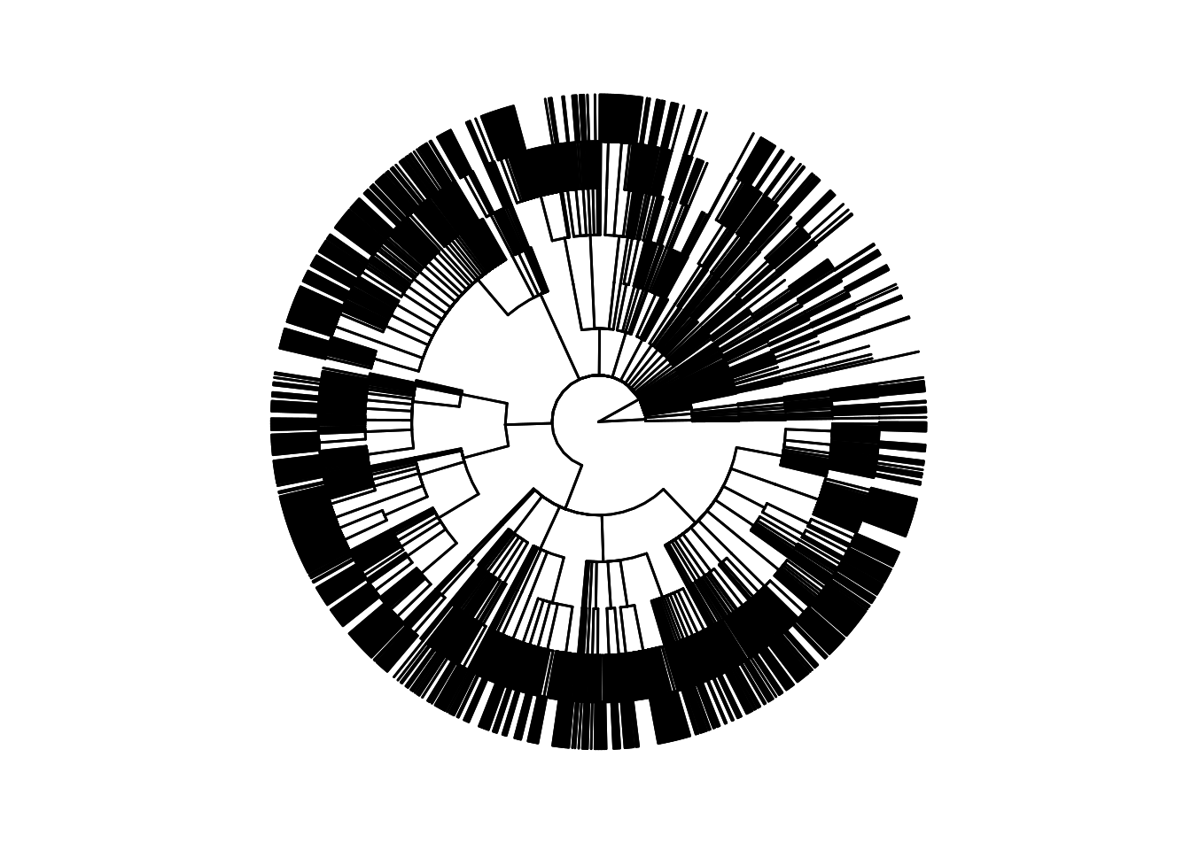
The plotRowTree() function from the miaViz package provides a convenient way to visualize the phylogeny.
library(miaViz)

plotRowTree(tse)
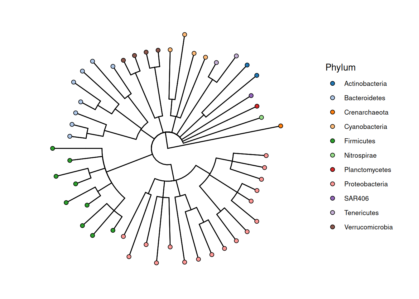
By default, the visualized phylogeny has only a limited amount of information. To enrich the visualization, we can prune the tree to genus level and visualize to which phyla these genera belong to.
# Agglomerate data and prune tree
tse <- agglomerateByRank(tse, rank = "Genus")

# Get top features
top <- getTop(tse, top = 50L)

# Plot
plotRowTree(
    tse[top, ],
    tip.colour.by = "Phylum"
)
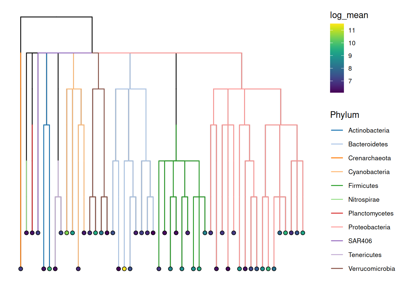
In addition to nodes and tips, we can also color edges based on feature metadata. Below, we color edges based on phyla and illustrate the mean abundance of genera by coloring tips. Moreover, we switch to a dendrogram layout with the help of the scater package.
library(scater)

# Calculate mean abundance
tse <- addPerFeatureQC(tse)
rowData(tse)[["log_mean"]] <- log(rowData(tse)[["mean"]])

# Plot
plotRowTree(
    tse[top, ],
    layout = "dendrogram",
    edge.colour.by = "Phylum",
    tip.colour.by = "log_mean"
)