3  Data containers

This section provides an introduction to TreeSummarizedExperiment (TreeSE) and MultiAssayExperiment (MAE) data containers introduced in Section 1.2. In microbiome data science, these containers link taxonomic abundance tables with rich side information on the taxa and samples. Taxonomic abundance data can be obtained by 16S rRNA amplicon or metagenomic sequencing, phylogenetic microarrays, or by other means. Many microbiome experiments include multiple versions and types of data generated independently or derived from each other through transformation or agglomeration. We start by providing recommendations on how to represent different varieties of multi-table data within the TreeSE class.

The options and recommendations are summarized in Table 3.1.

3.1 Structure of TreeSE

TreeSE contains several distinct slots, each holding a specific type of data. The assays slot is the core of TreeSE, storing abundance tables that contain the counts or concentrations of features in each sample. Features can be taxa, metabolites, antimicrobial resistance genes, or other measured entities, and are represented as rows. The columns correspond to unique samples.

Building upon the assays, TreeSE accommodates various data types for both features and samples. In rowData, the rows correspond to the same features (rows) as in the abundance tables, while the columns represent variables such as taxonomy ranks. Similarly, in colData, each row matches the samples (columns) from the abundance tables, with the columns of colData containing metadata like disease status or patient ID and time point if the dataset includes time series.

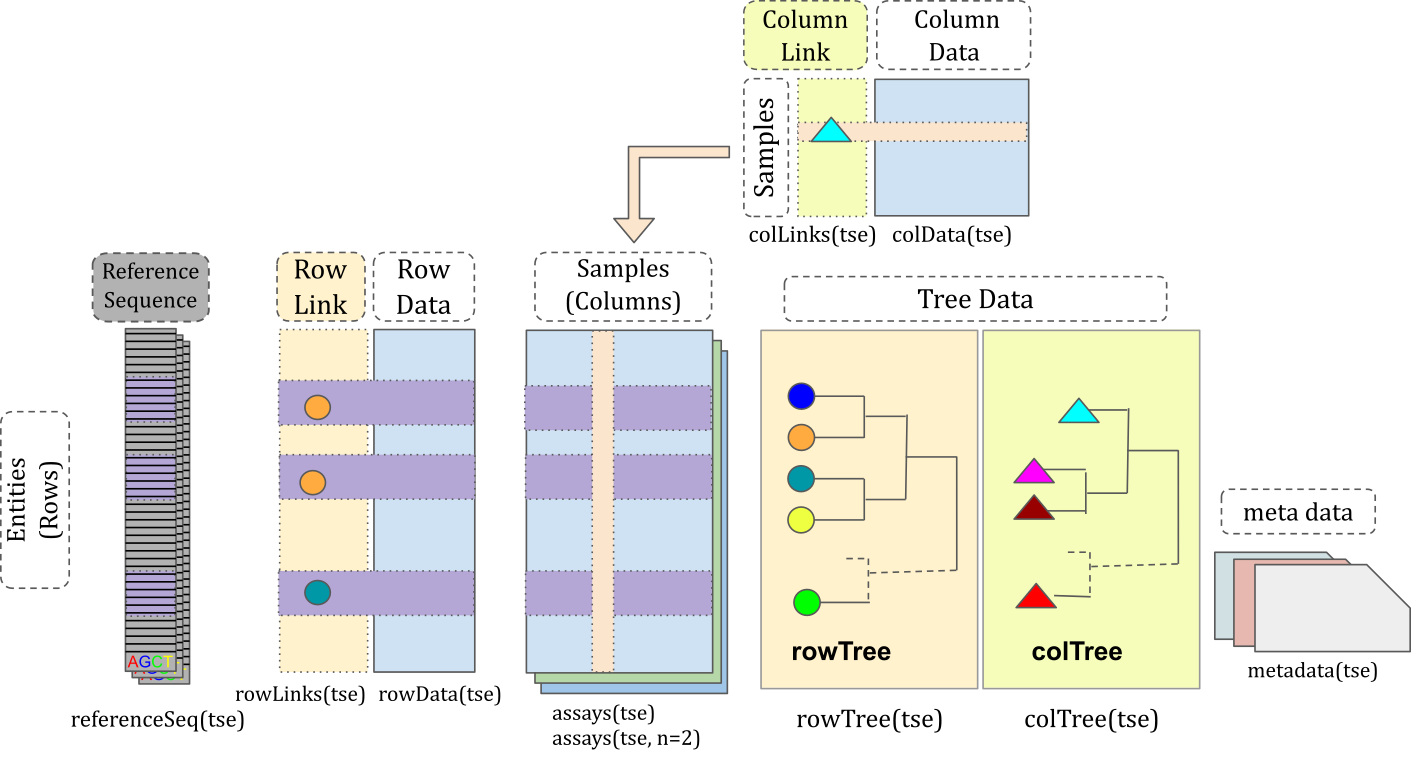
The slots in TreeSE are outlined below:

• assays: Stores a list of abundance tables. Each table has consistent rows and columns, where rows represent taxa and columns represent samples.
• rowData: Contains metadata about the rows (taxa). For example, this slot can include a taxonomy table.
• colData: Holds metadata about the columns (samples), such as patient information or the time points when samples were collected.
• rowTree: Stores a hierarchical tree for the rows, such as a phylogenetic tree representing the relationships between taxa.
• colTree: Includes a hierarchical tree for the columns, which can represent relationships between samples, for example, indicating whether patients are relatives and the structure of those relationships.
• rowLinks: Contains information about the linkages between rows and the nodes in the rowTree.
• colLinks: Contains information about the linkages between columns and the nodes in the colTree.
• referenceSeq: Holds reference sequences, i.e., the sequences that correspond to each taxon identified in the rows.
• metadata: Contains metadata about the experiment, such as the date it was conducted and the researchers involved.

These slots are illustrated in the figure below:

The structure of TreeSummarizedExperiment (TreeSE) object (Huang et al. 2021).

Huang, Ruizhu, Charlotte Soneson, Felix G. M. Ernst, et al. 2021. “TreeSummarizedExperiment: A S4 Class for Data with Hierarchical Structure [Version 2; Peer Review: 3 Approved].” F1000Research 9: 1246. https://doi.org/10.12688/f1000research.26669.2.

Additionally, TreeSE includes:

• reducedDim: Contains reduced dimensionality representations of the samples, such as Principal Component Analysis (PCA) results (see Chapter 14.
• altExp: Stores alternative experiments, which are TreeSE objects sharing the same samples but with different feature sets.

Among these, assays, rowData, colData, and metadata are shared with the SummarizedExperiment (SE) data container. reducedDim and altExp come from inheriting the SingleCellExperiment (SCE) class. The rowTree, colTree, rowLinks, colLinks, and referenceSeq slots are unique to TreeSE.

3.2 Rows and columns

Let us load example data and store it in variable tse.

library(mia)
data("GlobalPatterns", package = "mia")
tse <- GlobalPatterns
tse
##  class: TreeSummarizedExperiment 
##  dim: 19216 26 
##  metadata(0):
##  assays(1): counts
##  rownames(19216): 549322 522457 ... 200359 271582
##  rowData names(7): Kingdom Phylum ... Genus Species
##  colnames(26): CL3 CC1 ... Even2 Even3
##  colData names(7): X.SampleID Primer ... SampleType Description
##  reducedDimNames(0):
##  mainExpName: NULL
##  altExpNames(0):
##  rowLinks: a LinkDataFrame (19216 rows)
##  rowTree: 1 phylo tree(s) (19216 leaves)
##  colLinks: NULL
##  colTree: NULL

The TreeSE object, similar to a standard data.frame or matrix, has rows and columns. Typically, samples are stored in columns, while taxa (or features) are stored in rows. You can extract subsets of the data, such as the first five rows (first five taxa) and certain three columns (certain three samples). The object manages the linkages between data (e.g., the assay data and the sample metadata), ensuring that when you subset the data object, all its parts are subsetted simultaneously, such that they remain matched with each other.

tse <- tse[1:5, c(1, 19, 16)]
tse
##  class: TreeSummarizedExperiment 
##  dim: 5 3 
##  metadata(0):
##  assays(1): counts
##  rownames(5): 549322 522457 951 244423 586076
##  rowData names(7): Kingdom Phylum ... Genus Species
##  colnames(3): CL3 TRRsed1 NP2
##  colData names(7): X.SampleID Primer ... SampleType Description
##  reducedDimNames(0):
##  mainExpName: NULL
##  altExpNames(0):
##  rowLinks: a LinkDataFrame (5 rows)
##  rowTree: 1 phylo tree(s) (19216 leaves)
##  colLinks: NULL
##  colTree: NULL

Compared to the original data the dimensions are for rows and columns 5 and 3, respectively.

Note

SummarizedExperiment objects have rows and columns. Also MultiAssayExperiment, introduced in Section 3.8 have rows and cols but the structure is more complicated. You can find more examples on subsetting from Chapter 8.

3.3 Assay data

When studying microbiomes, the primary type of data is in the form of abundance of given microbes in given samples. This sample per taxa table forms the core of the TreeSE object, called the ‘The assay data’ .

An assay is a measurement of the presence and abundance of different microbial taxa in a sample. The assay data records this in a table where rows are unique taxa and columns are unique samples and each entry contains a number describing how many of a given taxon is present in a given sample. Note that when storing assays, the original data is count-based. However, due to the nature of how microbiome data is produced, these count-based abundances rarely reflect the true counts of microbial taxa in the sample, and thus the abundance tables often undergo different transformations, such as logarithmic, Centered Log-Ratio (CLR), or relative abundance to make these abundance values comparable with each other. SeeChapter 10 for more information on transformations.

The microbial abundance tables are stored in assays. The assays slot contains the abundance data as multiple count matrices. The result of assays is a list of matrices.

assays(tse)
##  List of length 1
##  names(1): counts

Individual assays can be accessed via assay.

assay(tse, "counts") |> head()
##         CL3 TRRsed1 NP2
##  549322   0       0   1
##  522457   0       0   0
##  951      0       0   0
##  244423   0       0   0
##  586076   0       0   0

So, in summary, in the world of microbiome analysis, an assay is essentially a way to describe the composition of microbes in a given sample. This way we can summarise the microbiome profile of a human gut or a sample of soil.

Furthermore, to illustrate the use of multiple assays, we can create an empty matrix and add it to the object.

mat <- matrix(nrow = nrow(tse), ncol = ncol(tse))
assay(tse, "empty_table", withDimnames=FALSE) <- mat
assays(tse)
##  List of length 2
##  names(2): counts empty_table

Now there are two assays available in the tse object, counts and empty_table.

assay(tse, "empty_table") |> head()
##         CL3 TRRsed1 NP2
##  549322  NA      NA  NA
##  522457  NA      NA  NA
##  951     NA      NA  NA
##  244423  NA      NA  NA
##  586076  NA      NA  NA

Here the dimension of the assay data remains unchanged. This is in fact a requirement for the assays.

3.4 colData

colData contains information about the samples used in the study. This sample metadata can include details such as the sample ID, the primers used in the analysis, the barcodes associated with the sample (truncated or complete), the type of sample (e.g. soil, fecal, mock) and a description of the sample.

colData(tse)
##  DataFrame with 3 rows and 7 columns
##          X.SampleID   Primer Final_Barcode Barcode_truncated_plus_T
##            <factor> <factor>      <factor>                 <factor>
##  CL3        CL3      ILBC_01        AACGCA                   TGCGTT
##  TRRsed1    TRRsed1  ILBC_22        ACATGT                   ACATGT
##  NP2        NP2      ILBC_19        ACAGTT                   AACTGT
##          Barcode_full_length         SampleType
##                     <factor>           <factor>
##  CL3             CTAGCGTGCGT Soil              
##  TRRsed1         CACGTGACATG Sediment (estuary)
##  NP2             TCGCGCAACTG Ocean             
##                                       Description
##                                          <factor>
##  CL3     Calhoun South Carolina Pine soil, pH 4.9
##  TRRsed1 Tijuana River Reserve, depth 1          
##  NP2     Newport Pier, CA surface water, Time 1

To illustrate, X.SampleID gives the sample identifier, SampleType indicates the sample type (e.g. soil, fecal matter, control) and Description provides an additional description of the sample.

3.5 rowData

rowData contains data on the features, such as microbial taxa of the analyzed samples. This is particularly important in the microbiome field for storing taxonomic information, such as the Species, Genus or Family of the different microorganisms present in samples. This taxonomic information is extremely important for understanding the composition and diversity of the microbiome in each sample.

rowData(tse)
##  DataFrame with 5 rows and 7 columns
##             Kingdom        Phylum        Class        Order        Family
##         <character>   <character>  <character>  <character>   <character>
##  549322     Archaea Crenarchaeota Thermoprotei           NA            NA
##  522457     Archaea Crenarchaeota Thermoprotei           NA            NA
##  951        Archaea Crenarchaeota Thermoprotei Sulfolobales Sulfolobaceae
##  244423     Archaea Crenarchaeota        Sd-NA           NA            NA
##  586076     Archaea Crenarchaeota        Sd-NA           NA            NA
##               Genus                Species
##         <character>            <character>
##  549322          NA                     NA
##  522457          NA                     NA
##  951     Sulfolobus Sulfolobusacidocalda..
##  244423          NA                     NA
##  586076          NA                     NA

3.6 rowTree

Phylogenetic trees play an important role in the microbiome field. Many times it is useful to know how closely related the microbial taxa present in the data are. For example, to calculate widely-used phylogenetically weighted microbiome dissimilarity metrics such as UniFrac and wUniFrac, we need information on not only the presence and abundance of microbial taxa in each sample but also the evolutionary relatedness among these taxa. The TreeSE class can keep track of relations among features (taxa) via two functions, rowTree and rowLinks.

A tree can be accessed via rowTree as phylo object.

rowTree(tse)
##  
##  Phylogenetic tree with 19216 tips and 19215 internal nodes.
##  
##  Tip labels:
##    549322, 522457, 951, 244423, 586076, 246140, ...
##  Node labels:
##    , 0.858.4, 1.000.154, 0.764.3, 0.995.2, 1.000.2, ...
##  
##  Rooted; includes branch lengths.

Each row in TreeSE is linked to a specific node in a tree. This relationship is stored in the rowLinks slot, which has the same rows as TreeSE. The rowLinks slot contains information about which tree node corresponds to each row and whether the node is a leaf (tip) or an internal node, among other details.

rowLinks(tse)
##  LinkDataFrame with 5 rows and 5 columns
##        nodeLab   nodeNum nodeLab_alias    isLeaf   whichTree
##    <character> <integer>   <character> <logical> <character>
##  1      549322         1       alias_1      TRUE       phylo
##  2      522457         2       alias_2      TRUE       phylo
##  3         951         3       alias_3      TRUE       phylo
##  4      244423         4       alias_4      TRUE       phylo
##  5      586076         5       alias_5      TRUE       phylo

Please note that there can be a 1:1 relationship between tree nodes and features, but this is not a must-have. This means there can be features that are not linked to nodes, and nodes that are not linked to features. To change the links in an existing object, the changeTree() function is available.

3.7 Alternative Experiments

Alternative experiments (altExp) complement assays. They can contain complementary data, which is no longer tied to the same dimensions as the assay data. However, the number of samples (columns) must be the same.

This can come into play, for instance, when one has taxonomic abundance profiles quantified using different measurement technologies, such as phylogenetic microarrays, amplicon sequencing, or metagenomic sequencing. Another common use case is including abundance tables for different taxonomic ranks. Such alternative experiments concerning the same set of samples can be stored as

1. Separate assays assuming that the taxonomic information can be mapped between features directly 1:1; or
2. Data in the altExp slot of the TreeSE, if the feature dimensions differ. Each element of the altExp slot is a SE or an object from a derived class with independent feature data.

The following shows how to store taxonomic abundance tables agglomerated at different taxonomic levels. However, the data could as well originate from entirely different measurement sources (e.g., 16S amplicon and metagenomic sequence data) as long as the samples match.

Let us first subset the data so that it has only two rows.

tse_sub <- tse[1:2, ]
# Both have the same number of columns (samples)
dim(tse)
##  [1] 5 3
dim(tse_sub)
##  [1] 2 3

Then we can add the new data object as an alternative experiment in the original data.

# Add the new data object to the original data object as an alternative
# experiment with the specified name
altExp(tse, "subsetted") <- tse_sub

# Retrieve and display the names of alternative experiments available
altExpNames(tse)
##  [1] "subsetted"

Now, if we subset the data, this acts on both the altExp and the assay data.

tse_single_sample <- tse[, 1]
dim(altExp(tse_single_sample,"subsetted"))
##  [1] 2 1

For more details on altExp, you can check the introduction to the SingleCellExperiment package (Lun and Risso 2020).

Lun, Aaron, and Davide Risso. 2020. SingleCellExperiment: S4 Classes for Single Cell Data.

3.8 Multiple experiments

Multiple experiments relate to complementary measurement types from the same samples, such as transcriptomic or metabolomic profiling of the microbiome. Multiple experiments can be represented using the same options as alternative experiments, or by using the MAE class (Ramos et al. 2017). Depending on how the datasets relate to each other the data can be stored as:

1. altExp if the samples can be matched directly 1:1; or
2. As MAE objects, in which the connections between samples are defined through a sampleMap. Each element on the ExperimentList of an MAE is matrix or matrix-like objects, including SE objects, and the number of samples can differ between the elements.

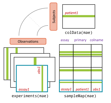
In a MAE, the “subjects” represent patients. The MAE has four main slots, with experiments being the core. This slot holds a list of experiments, each in (Tree)SE format. To handle complex mappings between samples (observations) across different experiments, the sampleMap slot stores information about how each sample in the experiments is linked to a patient. Metadata for each patient is stored in the colData slot. Unlike the colData in TreeSE, this colData is meant to store only metadata that remains constant throughout the trial.

• experiments: Contains experiments, such as different omics data, in TreeSE format.
• sampleMap: Holds linkages between patients (subjects) and samples in the experiments (observations).
• colData: Includes patient metadata that remains unchanged throughout the trial.

These slots are illustrated in the figure below:

The structure of MultiAssayExperiment (MAE) object (Ramos et al. 2017).

Ramos, Marcel, Lucas Schiffer, Angela Re, Rimsha Azhar, Azfar Basunia, Carmen Rodriguez Cabrera, Tiffany Chan, et al. 2017. “Software for the Integration of Multiomics Experiments in Bioconductor.” Cancer Research. https://doi.org/10.1158/0008-5472.CAN-17-0344.

Additionally, the object includes a metadata slot that contains information about the dataset, such as the trial period and the creator of the MAE object.

The MAE object can handle more complex relationships between experiments. It manages the linkages between samples and experiments, ensuring that the data remains consistent and well-organized.

data("HintikkaXOData")
mae <- HintikkaXOData
mae
##  A MultiAssayExperiment object of 3 listed
##   experiments with user-defined names and respective classes.
##   Containing an ExperimentList class object of length 3:
##   [1] microbiota: TreeSummarizedExperiment with 12706 rows and 40 columns
##   [2] metabolites: TreeSummarizedExperiment with 38 rows and 40 columns
##   [3] biomarkers: TreeSummarizedExperiment with 39 rows and 40 columns
##  Functionality:
##   experiments() - obtain the ExperimentList instance
##   colData() - the primary/phenotype DataFrame
##   sampleMap() - the sample coordination DataFrame
##   `$`, `[`, `[[` - extract colData columns, subset, or experiment
##   *Format() - convert into a long or wide DataFrame
##   assays() - convert ExperimentList to a SimpleList of matrices
##   exportClass() - save data to flat files

The sampleMap is a crucial component of the MAE object as it acts as an important bookkeeper, maintaining the information about which samples are associated with which experiments. This ensures that data linkages are correctly managed and preserved across different types of measurements.

sampleMap(mae) |> head()
##  DataFrame with 6 rows and 3 columns
##         assay     primary     colname
##      <factor> <character> <character>
##  1 microbiota          C1          C1
##  2 microbiota          C2          C2
##  3 microbiota          C3          C3
##  4 microbiota          C4          C4
##  5 microbiota          C5          C5
##  6 microbiota          C6          C6

For illustration, let’s subset the data by taking first five samples.

mae <- mae[ , 1:5, ]
mae
##  A MultiAssayExperiment object of 3 listed
##   experiments with user-defined names and respective classes.
##   Containing an ExperimentList class object of length 3:
##   [1] microbiota: TreeSummarizedExperiment with 12706 rows and 5 columns
##   [2] metabolites: TreeSummarizedExperiment with 38 rows and 5 columns
##   [3] biomarkers: TreeSummarizedExperiment with 39 rows and 5 columns
##  Functionality:
##   experiments() - obtain the ExperimentList instance
##   colData() - the primary/phenotype DataFrame
##   sampleMap() - the sample coordination DataFrame
##   `$`, `[`, `[[` - extract colData columns, subset, or experiment
##   *Format() - convert into a long or wide DataFrame
##   assays() - convert ExperimentList to a SimpleList of matrices
##   exportClass() - save data to flat files

Note

If you have multiple experiments containing multiple measures from same sources (e.g., patients/host, individuals/sites), you can utilize the MultiAssayExperiment object to keep track of which samples belong to which patient.

The following dataset illustrates how to utilize the sample mapping system in MAE. It includes two omics data: biogenic amines and fatty acids, collected from 10 chickens.

mae <- readRDS(system.file("extdata", "mae_holofood.Rds", package = "OMA"))
mae
##  A MultiAssayExperiment object of 2 listed
##   experiments with user-defined names and respective classes.
##   Containing an ExperimentList class object of length 2:
##   [1] BIOGENIC AMINES: TreeSummarizedExperiment with 7 rows and 14 columns
##   [2] FATTY ACIDS: TreeSummarizedExperiment with 19 rows and 19 columns
##  Functionality:
##   experiments() - obtain the ExperimentList instance
##   colData() - the primary/phenotype DataFrame
##   sampleMap() - the sample coordination DataFrame
##   `$`, `[`, `[[` - extract colData columns, subset, or experiment
##   *Format() - convert into a long or wide DataFrame
##   assays() - convert ExperimentList to a SimpleList of matrices
##   exportClass() - save data to flat files

We can see that there are more than ten samples per omic dataset due to multiple samples from different time points collected for some animals. From the colData of MAE, we can observe the individual animal metadata, including information that remains constant throughout the trial.

colData(mae)
##  DataFrame with 10 rows and 13 columns
##                 marker.canonical_url         marker.type Treatment code
##                            <numeric>              <list>    <character>
##  SAMEA112904734                   NA TREATMENT,TRIAL,PEN             CO
##  SAMEA112904735                   NA TREATMENT,TRIAL,PEN             CC
##  SAMEA112904737                   NA TREATMENT,TRIAL,PEN             CC
##  SAMEA112904741                   NA TREATMENT,TRIAL,PEN             CC
##  SAMEA112904746                   NA TREATMENT,TRIAL,PEN             CC
##  SAMEA112904748                   NA TREATMENT,TRIAL,PEN             CO
##  SAMEA112904749                   NA TREATMENT,TRIAL,PEN             CC
##  SAMEA112904755                   NA TREATMENT,TRIAL,PEN             CC
##  SAMEA112904762                   NA TREATMENT,TRIAL,PEN             CO
##  SAMEA112904763                   NA TREATMENT,TRIAL,PEN             CC
##                 Treatment name  Trial code Trial description   Trial end
##                    <character> <character>       <character> <character>
##  SAMEA112904734      Probiotic          CB           Trial 2  2019-05-19
##  SAMEA112904735        Control          CC           Trial 3  2019-07-14
##  SAMEA112904737        Control          CB           Trial 2  2019-05-19
##  SAMEA112904741        Control          CC           Trial 3  2019-07-14
##  SAMEA112904746        Control          CB           Trial 2  2019-05-19
##  SAMEA112904748      Probiotic          CC           Trial 3  2019-07-14
##  SAMEA112904749        Control          CA           Trial 1  2019-03-11
##  SAMEA112904755        Control          CB           Trial 2  2019-05-19
##  SAMEA112904762      Probiotic          CC           Trial 3  2019-07-14
##  SAMEA112904763        Control          CA           Trial 1  2019-03-11
##                 Trial start         animal      system          canonical_url
##                 <character>    <character> <character>            <character>
##  SAMEA112904734  2019-04-21 SAMEA112904734     chicken https://www.ebi.ac.u..
##  SAMEA112904735  2019-06-09 SAMEA112904735     chicken https://www.ebi.ac.u..
##  SAMEA112904737  2019-04-21 SAMEA112904737     chicken https://www.ebi.ac.u..
##  SAMEA112904741  2019-06-09 SAMEA112904741     chicken https://www.ebi.ac.u..
##  SAMEA112904746  2019-04-21 SAMEA112904746     chicken https://www.ebi.ac.u..
##  SAMEA112904748  2019-06-09 SAMEA112904748     chicken https://www.ebi.ac.u..
##  SAMEA112904749  2019-02-04 SAMEA112904749     chicken https://www.ebi.ac.u..
##  SAMEA112904755  2019-04-21 SAMEA112904755     chicken https://www.ebi.ac.u..
##  SAMEA112904762  2019-06-09 SAMEA112904762     chicken https://www.ebi.ac.u..
##  SAMEA112904763  2019-02-04 SAMEA112904763     chicken https://www.ebi.ac.u..
##                 Average Daily Feed intake: Day 00 - 07
##                                              <numeric>
##  SAMEA112904734                                  19.39
##  SAMEA112904735                                  22.35
##  SAMEA112904737                                  18.18
##  SAMEA112904741                                  21.68
##  SAMEA112904746                                  19.75
##  SAMEA112904748                                  21.10
##  SAMEA112904749                                  18.67
##  SAMEA112904755                                  23.36
##  SAMEA112904762                                  21.15
##  SAMEA112904763                                  19.67
##                 Average Daily Feed intake: Day 00 - 07, unit
##                                                  <character>
##  SAMEA112904734                                            g
##  SAMEA112904735                                            g
##  SAMEA112904737                                            g
##  SAMEA112904741                                            g
##  SAMEA112904746                                            g
##  SAMEA112904748                                            g
##  SAMEA112904749                                            g
##  SAMEA112904755                                            g
##  SAMEA112904762                                            g
##  SAMEA112904763                                            g

The sampleMap slot now contains mappings between each unique sample and the corresponding individual animal. There are as many rows as there are total samples.

The “colname” column refers to the samples in the omic dataset identified in the “assay” column, while the “primary” column provides information about the animals. You will notice that some animals are listed multiple times, reflecting the multiple omics and time points collected for those individuals.

sampleMap(mae)
##  DataFrame with 33 rows and 3 columns
##                assay        primary        colname
##             <factor>    <character>    <character>
##  1   BIOGENIC AMINES SAMEA112904734 SAMEA112906114
##  2   BIOGENIC AMINES SAMEA112904734 SAMEA112906592
##  3   BIOGENIC AMINES SAMEA112904735 SAMEA112906338
##  4   BIOGENIC AMINES SAMEA112904735 SAMEA112906810
##  5   BIOGENIC AMINES SAMEA112904737 SAMEA112906123
##  ...             ...            ...            ...
##  29      FATTY ACIDS SAMEA112904755 SAMEA112906112
##  30      FATTY ACIDS SAMEA112904755 SAMEA112906590
##  31      FATTY ACIDS SAMEA112904762 SAMEA112906315
##  32      FATTY ACIDS SAMEA112904762 SAMEA112906787
##  33      FATTY ACIDS SAMEA112904763 SAMEA112905916

For information have a look at the intro vignette of the MultiAssayExperiment package.

Recommended options for storing multiple data tables in microbiome studies

Table 3.1: The assays are best suited for data transformations (one-to-one match between samples and columns across the assays). The alternative experiments are particularly suitable for alternative versions of the data that are of same type but may have a different number of features (e.g. taxonomic groups); this is for instance the case with taxonomic abundance tables agglomerated at different levels (e.g. genus vs. phyla) or alternative profiling technologies (e.g. amplicon sequencing vs. shallow shotgun metagenomics). For alternative experiments one-to-one match between samples (cols) is libraryd but the alternative experiment tables can have different numbers of features (rows). Finally, elements of the MAE provide the most flexible way to incorporate multi-omic data tables with flexible numbers of samples and features. We recommend these conventions as the basis for methods development and application in microbiome studies.

Option	Rows (features)	Cols (samples)	Recommended
assays	match	match	Data transformations
altExp	free	match	Alternative experiments
MultiAssay	free	free (mapping)	Multi-omic experiments

Multi-assay analyses, discussed in sections Section 20.1 and Chapter 21, can be facilitated by the multi-assay data containers, TreeSummarizedExperiment and MultiAssayExperiment. These are scalable and contain different types of data in a single container, making this framework particularly suited for multi-assay microbiome data incorporating different types of complementary data sources in a single, reproducible workflow. An alternative experiment can be stored in altExp slot of the SE data container. Alternatively, both experiments can be stored side-by-side in an MAE data container.