22 Ordination-based multiassay analysis

In this chapter, we continue from where we left off in the previous section (referenced as Section 21.1). Specifically, we introduce an analytical method called Multi-Omics Factor Analysis. This method is described as “ordination-based,” meaning it involves techniques that reduce the dimensionality of the data while preserving as much variability as possible. Ordination methods are often used in multivariate analysis to visualize patterns, trends, and relationships in complex data sets, making them particularly useful for multi-omics data where multiple types of biological data are integrated and analyzed together.

See Chapter 14 for more information on ordination methods.

22.1 Multi-Omics Factor Analysis

Multi-Omics Factor Analysis (MOFA) is an unsupervised method for integrating multi-omic data sets in a downstream analysis (Argelaguet 2018). It could be seen as a generalization of principal component analysis. Yet, with the ability to infer a latent (low-dimensional) representation, shared among the multiple (-omics) data sets in hand.

Argelaguet, Ricard et al. 2018. “Multi-Omics Factor Analysis—a Framework for Unsupervised Integration of Multi-Omics Data Sets.” Molecular Systems Biology 14 (6): e8124. https://doi.org/10.15252/msb.20178124.

We use the R MOFA2 package for the analysis, and install the corresponding dependencies.

library(mia)
# Load the data
data(HintikkaXOData, package = "mia")
mae <- HintikkaXOData

The mae object could be used straight to create the MOFA model. Yet, we transform our assays since the model assumes normality per default, and Gaussian model is recommended (see MOFA2 FAQ). However, Poisson and Bernoulli distribution models are also offered.

Note that duplicates, such as “uncultured”, might appear when aggregating the microbiome data by a taxonomic rank. To check for duplicates, run any(duplicated(rownames(mae[[1]]))). If it returns TRUE, then the duplicates are present. We can add rownames(mae[[1]]) <- getTaxonomyLabels(mae[[1]], make.unique=TRUE) to remove them.

To run MOFA2, it needs to connect mofapy2 Python packages via the reticulate package, as clarified in the MOFA2 vignette.

The following chunk checks if Python dependencies are already installed, and installs them if they are not available. If this setup causes issues, update miniconda and mofapy2.

library(reticulate)

# Set miniconda environment
if( !reticulate:::miniconda_exists() ){
    install_miniconda()
}
##  [1] "/root/.local/share/r-miniconda"
if( !condaenv_exists(miniconda_path()) ){
    use_miniconda(condaenv = miniconda_path(), required = FALSE)
}

# Check if mofapy2 is installed, and install it if not
if( !py_module_available("mofapy2") ){
    py_install(
        packages = "mofapy2",
        pip = TRUE,
        pip_ignore_installed = TRUE,
    )
}

library(MOFA2)
# For simplicity, classify all high-fat diets as high-fat, and all the low-fat
# diets as low-fat diets
colData(mae)$Diet <- ifelse(
    colData(mae)$Diet == "High-fat" | colData(mae)$Diet == "High-fat + XOS",
    "High-fat", "Low-fat")

# Agglomerate microbiome data
mae[[1]] <- agglomerateByPrevalence(mae[[1]], rank = "Genus")
# Transforming microbiome data with clr and by scaling
mae[[1]] <- transformAssay(mae[[1]], method = "clr", pseudocount = TRUE)
mae[[1]] <- transformAssay(
    mae[[1]], assay.type = "clr", method = "standardize", MARGIN = "rows")

# Transforming metabolomic data with log10 and by scaling
mae[[2]] <- transformAssay(mae[[2]], assay.type = "nmr", method = "log10")
mae[[2]] <- transformAssay(
    mae[[2]], assay.type = "log10", method = "standardize")

# Transforming biomarker data by scaling
mae[[3]] <- transformAssay(
    mae[[3]], assay.type = "signals", method = "standardize", MARGIN = "rows")

# Removing the assays no longer needed
assays(mae[[1]]) <- assays(mae[[1]])["standardize"]
assays(mae[[2]]) <- assays(mae[[2]])["standardize"]
assays(mae[[3]]) <- assays(mae[[3]])["standardize"]

# Building our mofa model
model <- create_mofa_from_MultiAssayExperiment(
    mae,
    groups = "Diet",
    extract_metadata = TRUE)
model
##  Untrained MOFA model with the following characteristics: 
##   Number of views: 3 
##   Views names: microbiota metabolites biomarkers 
##   Number of features (per view): 112 38 39 
##   Number of groups: 2 
##   Groups names: High-fat Low-fat 
##   Number of samples (per group): 20 20 
##

Model options can be defined as follows:

model_opts <- get_default_model_options(model)
model_opts$num_factors <- 5
model_opts |> head()
##  $likelihoods
##   microbiota metabolites  biomarkers 
##   "gaussian"  "gaussian"  "gaussian" 
##  
##  $num_factors
##  [1] 5
##  
##  $spikeslab_factors
##  [1] FALSE
##  
##  $spikeslab_weights
##  [1] FALSE
##  
##  $ard_factors
##  [1] TRUE
##  
##  $ard_weights
##  [1] TRUE

Training options for the model are defined in the following way:

train_opts <- get_default_training_options(model)
train_opts |> head()
##  $maxiter
##  [1] 1000
##  
##  $convergence_mode
##  [1] "fast"
##  
##  $drop_factor_threshold
##  [1] -1
##  
##  $verbose
##  [1] FALSE
##  
##  $startELBO
##  [1] 1
##  
##  $freqELBO
##  [1] 5

The model is then prepared with prepare_mofa() and trained with run_mofa():

model <- prepare_mofa(
  object = model,
  model_options = model_opts
)

# Some systems may require the specification `use_basilisk = TRUE`
# so it has been added to the following code
model <- run_mofa(model, use_basilisk = TRUE)

The explained variance is visualized with the plot_variance_explained() function.

library(patchwork)
library(ggplot2)

plot_list <- plot_variance_explained(
    model,
    x = "view", y = "factor",
    plot_total = TRUE)

wrap_plots(plot_list, nrow = 2) +
    plot_annotation(
        title = "Variance Explained per factor and assay",
        theme = theme(plot.title = element_text(hjust = 0.5)))

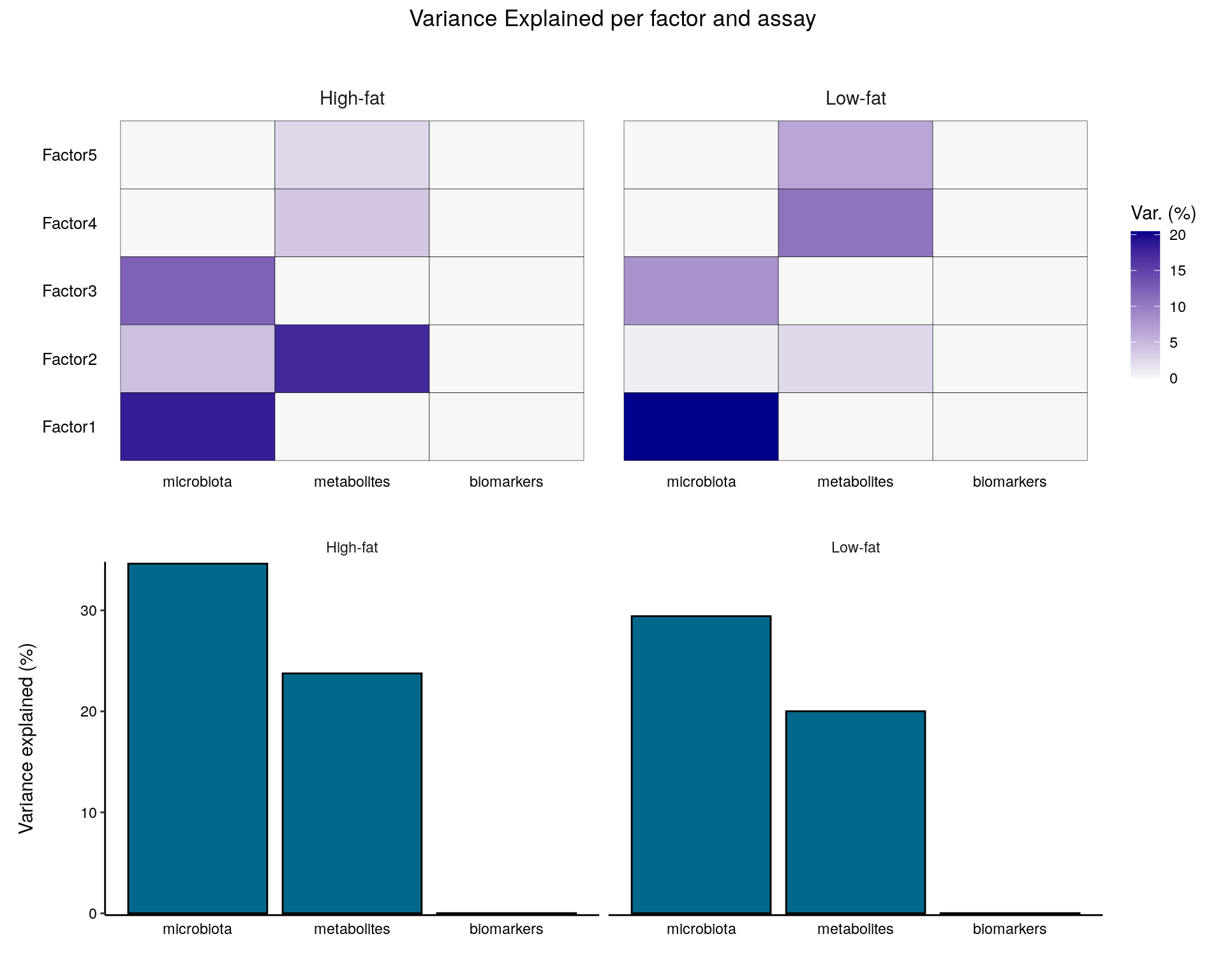
From the plot, we can observe that the microbiota accounts for most of the variability in the data. Biomarkers do not significantly explain the variability. The variability in the microbiota is primarily captured in factors 1 and 2, while metabolites are primarily represented in factor 2.

We can then visualize the top weights for microbiota and metabolites for the first two factors to analyze co-varying features.

plot_list <- lapply(
    c("microbiota", "metabolites"),
    plot_top_weights,
    object = model,
    factors = c(1, 2),
    nfeatures = 10
    )

wrap_plots(plot_list, ncol = 1) & theme(text = element_text(size = 8))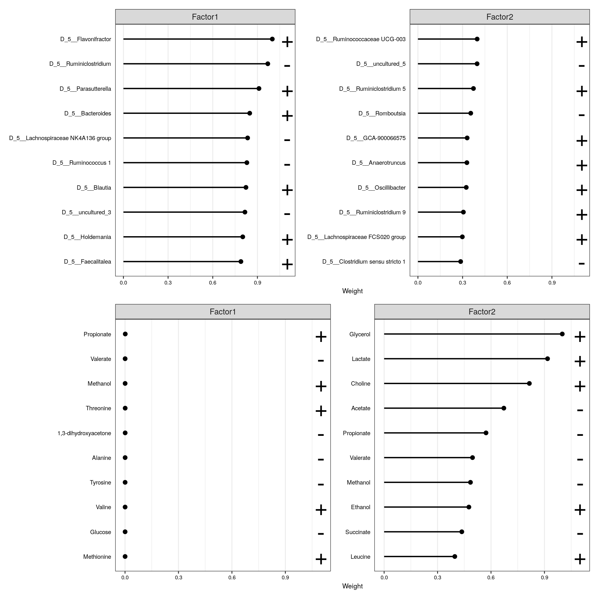

From the visualization, we can see that glycerol, lactate, and choline are positively associated with factor 2, while acetate is negatively associated among the metabolites. In terms of microbiota, Ruminococcaceae and Ruminodostridium, for instance, are positively associated with the same factor. This indicates that these features co-vary in the data, suggesting a positive association with glycerol, lactate, and choline, and a negative association with acetate and these microbes.

More tutorials and examples of using the package are found at MOFA2 tutorials.

Exercises

Goal: After completing these exercises, you should be able to run and interpret MOFA results.

Exercise 1: MOFA

Load any of the example datasets in MultiAssayExperiment format mentioned in Section 4.2.
Agglomerate microbiota data to prevalent phyla.
Apply CLR transformation to microbiota data.
Apply relative transformation and log10 transformation to other metabolite or other omic.
Create MOFA2 object from the MultiAssayExperiment.
Run MOFA.
Visualize the explained variance. How much variance is explained in total, and which omic accounts the most variance?
For each omic, visualize the features with the largest weights. Can you identify features that are co-varying?
If you completed exercises in Section 21.1, did you get similar results? Do the co-varying features also exhibited correlation?

Useful functions:

data(), agglomerateByPrevalence, transformAssay(), MOFA2::create_mofa_from_MultiAssayExperiment(), MOFA2::run_mofa(), MOFA2::plot_variance_explained(), MOFA2::plot_top_weights(), getCrossAssociation(), ComplexHeatmap::Heatmap()