1  Microbiome data science in Bioconductor

This work - Orchestrating Microbiome Analysis with Bioconductor (Tuomas Borman et al. 2024) - contributes novel methods and educational resources for microbiome data science. It aims to teach the grammar of Bioconductor workflows in the context of microbiome data science. We show, through concrete examples, how to use the latest developments and data analytical strategies in R/Bioconductor for the manipulation, analysis, and reproducible reporting of hierarchical, heterogeneous, and multi-modal microbiome profiling data. The data science methodology is tightly integrated with the broader R/Bioconductor ecosystem. The support for modularity and interoperability is key to efficient resource sharing and collaborative development both within and across research fields.

Tuomas Borman, Leo Lahti, Sudarshan Shetty, Felix M Ernst, et al. 2024. Orchestrating Microbiome Analysis with Bioconductor [Beta Version]. microbiome.github.io/oma/.

1.1 Bioconductor

Bioconductor is a project that focuses on the development of high-quality open research software for life sciences (Gentleman et al. 2004; Huber et al. 2015). The software packages are primarily coded in R, and they undergo continuous testing and peer review to ensure high quality.

Gentleman, Robert C, Vincent J Carey, Douglas M Bates, Ben Bolstad, Marcel Dettling, Sandrine Dudoit, Byron Ellis, et al. 2004. “Bioconductor: Open Software Development for Computational Biology and Bioinformatics.” Genome Biology 5: R80.
Huber, W., V. J. Carey, R. Gentleman, S. Anders, M. Carlson, B. S. Carvalho, H. C. Bravo, et al. 2015. Orchestrating High-Throughput Genomic Analysis with Bioconductor.” Nature Methods 12 (2): 115–21. http://www.nature.com/nmeth/journal/v12/n2/full/nmeth.3252.html.

Bioconductor logo.

Central to the software in Bioconductor are data containers, which provide a structured presentation of data. A data container consists of slots that are dedicated to certain type of data, for example, to abundance table and sample metadata. Biological data is often complex and multidimensional, making data containers particularly beneficial. There are several key advantages to using data containers:

  • Ease of handling: Data subsetting and bookkeeping become more straightforward.
  • Development efficiency: Developers can create efficient methods, knowing the data will be in a consistent format.
  • User accessibility: Users can easily apply complex methods to their data.

The most common data container in Bioconductor is SummarizedExperiment. It is further expanded to fulfill needs of certain application field. SummarizedExperiment and its derivatives, have already been widely adopted in microbiome research, single cell sequencing, and in other fields, allowing rapid adoption and the extension of emerging data science techniques across application domains. See Section 2.1 for more details on how to handle data containers from the SummarizedExperiment family.

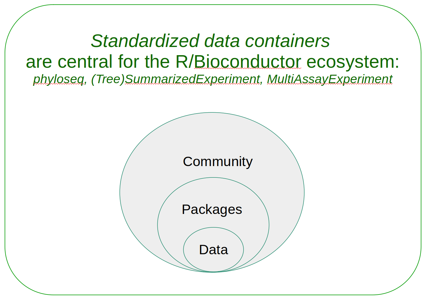
The Bioconductor microbiome data science framework consists of:

  • Data containers, designed to organize multi-assay microbiome data
  • R/Bioconductor packages that provide dedicated methods
  • Community of users and developers

Data containers are central in Bioconductor.

1.2 Microbiome data science in Bioconductor

While microbiota is used to refer micro-organisms within well-specified area, microbiome means microbiota and their genetic material (Marchesi and Ravel 2015). Because the complex nature of the microbiome data, computational methods are essential in microbiome research.

Marchesi, Julian R., and Jacques Ravel. 2015. “The Vocabulary of Microbiome Research: A Proposal.” Microbiome 3 (1). https://doi.org/10.1186/s40168-015-0094-5.
McMurdie, PJ, and S Holmes. 2013. Phyloseq: An r Package for Reproducible Interactive Analysis and Graphics of Microbiome Census Data.” PLoS ONE 8: e61217. https://doi.org/10.1371/journal.pone.0061217.

The phyloseq data container has been dominant in the microbiome field within Bioconductor over the past decade (McMurdie and Holmes 2013). However, there has been a growing popularity of tools based on the SummarizedExperiment framework.

An optimal data container should efficiently store and manage large volumes of data, including modified or transformed copies. Furthermore, it should seamlessly integrate into the broader ecosystem of Bioconductor, minimizing duplication of effort and facilitating interoperability with other tools and packages.

Optimal data container.

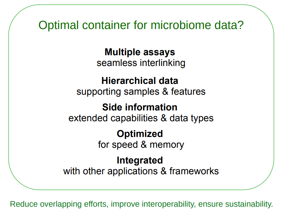
TreeSummarizedExperiment was developed to address these requirements (Huang et al. 2021). The miaverse framework was subsequently built around the TreeSummarizedExperiment data container Chapter 2.

Huang, Ruizhu, Charlotte Soneson, Felix G. M. Ernst, et al. 2021. “TreeSummarizedExperiment: A S4 Class for Data with Hierarchical Structure [Version 2; Peer Review: 3 Approved].” F1000Research 9: 1246. https://doi.org/10.12688/f1000research.26669.2.

1.3 Open data science

Open data science emphasizes sharing code and, where feasible, data alongside results (Shetty and Lahti 2019). Utilizing Bioconductor tools facilitates the development of efficient and reproducible data science workflows. Enhanced transparency in research accelerates scientific progress. As open science is a fundamental concept in microbiome research, this book aims to educate readers about reproducible reporting practices.

Shetty, Sudarshan, and Leo Lahti. 2019. “Microbiome Data Science.” Journal of Biosciences 44: 115. https://doi.org/10.1007/s12038-019-9930-2.
Summary
  • Bioconductor is a large ecosystem for bioinformatics.
  • Data containers are fundamental in Bioconductor.
  • SummarizedExperiment is the most common data container in Bioconductor.
Exercises

Exercise 1: Introduction to Bioconductor

Goal: Learn how to navigate Bioconductor website and get idea on the available packages.

  1. Go to Bioconductor website.
  2. Navigate to “Packages” section.
  3. Search for packages with the biocViews category “microbiome”. How many different packages are available?
  4. Look up the mia package. What is its current version? Is it released or devel version?
  5. Locate the mia package’s Reference Manual. When was it last updated?

Reproducible reporting with Quarto

Before starting, read the Quarto guidelines for RStudio. This will help you understand the basics.

Exercise 2: Creating a Quarto Document

Goal: Learn how to create a Quarto document, add text, and structure content with Markdown.

  1. Open RStudio and create a new Quarto file.
  2. In the YAML metadata section at the top, change title: Untitled to title: "My First Quarto".
  3. Add a section with the heading # My first section and write a short paragraph underneath.
  4. Add a subsection ## List of items and create:
    • An ordered list (e.g., 1. First item)
    • An unordered list (e.g., - Bullet point)
  5. Add another subsection ## Link to web and create a link to the OMA book using [text](url).
  6. Click Render and check how your document looks.

Expected Outcome: A properly structured Quarto document with headings, lists, and a clickable link.

Exercise 3: Adding code chunks

Goal: Learn how to integrate R code within a Quarto document.

  1. Open RStudio and create a new Quarto file.

  2. Insert a code chunk by pressing Alt + Cmd + I (Mac) or Ctrl + Alt + I (Windows, Linux) or from navigation bar.

  3. Inside the chunk, define:

    A <- "my name"
    B <- 0
  4. Above the chunk, write: Below is my first code chunk.

  5. Insert another chunk below and modify B:

    B <- B + 100
  6. Add a name for this the chunk: Below I change variable B.

  7. Display A and B dynamically in text using inline R code. For example, you can write “My name is A and I have B dogs”, where A and B are the variables above thus automatically updating the text based on their values.

Expected Outcome: Rendered document showing code execution, and dynamic text updates.

Exercise 4: Customizing code chunk output

Goal: Learn to control visibility and formatting of code chunks.

  1. Create a new Quarto file.

  2. Insert three labeled code chunks (first_chunk, fig-box, tbl-coldata).

  3. Copy-paste the following code:

    #| label: first_chunk
    #| code-fold: true
    #| code-summary: "Show the code"
    x <- 1:10
    y <- x^2
    #| label: fig-box
    #| fig-width: 10
    plot(x, y)
    #| label: tbl-coldata
    #| echo: false
    data.frame(x, y)
  4. Render and observe:

    • The code of first chunk is folded.
    • The figure is wider.
    • The table appears without showing its generating code.
  5. Add fig-cap and tab-cap options.

  6. Cross-reference the figure using @fig-box.

Expected Outcome: Cleaner output with formatted figures and tables.

Back to top