9 Subsetting
In this chapter, we explore the concept of subsetting. Subsetting or filtering is the process of selecting specific rows or columns from a dataset based on certain criteria. When you subset your data, you retain the original values of the selected data points. For example, if you have a dataset of taxonomic features and you choose to keep only certain species, you still have the individual counts for those species. This allows you to analyze the data in detail, but you may lose information about other species that are not included.
Subsetting data helps to draw the focus of an analysis on particular sets of samples and / or features. When dealing with large datasets, the subset of interest can be extracted and investigated separately. This might improve performance and reduce the computational load.
Let us store GlobalPatterns into tse and check its original number of features (rows) and samples (columns).
When subsetting by sample, expect the number of columns to decrease. When subsetting by feature, expect the number of rows to decrease.
9.1 Subset by sample (column-wise)
Several criteria can be used to subset by sample:
- origin
- sampling time
- sequencing method
- DNA / RNA barcode
- cohort
For the sake of demonstration, here we will extract a subset containing only the samples of human origin (feces, skin or tongue), stored as SampleType within colData(tse) as well as in tse.
First, we would like to see all the possible values that SampleType can have and how frequent those are:
| Var1 | Freq |
|---|---|
| Feces | 4 |
| Freshwater | 2 |
| Freshwater (creek) | 3 |
| Mock | 3 |
| Ocean | 3 |
| Sediment (estuary) | 3 |
| Skin | 3 |
| Soil | 3 |
| Tongue | 2 |
Next, we logical index across the columns of tse (make sure to leave the first index empty to select all rows) and filter for the samples of human origin. For this, we use the information on the samples from the metadata colData(tse).
After subsetting, expect the number of columns to equal the sum of the frequencies of the samples that you are interested in. For instance, ncols = Feces + Skin + Tongue = 4 + 3 + 2 = 9.
9.2 Subset by feature (row-wise)
Similarly, here we will extract a subset containing only the features that belong to the phyla Actinobacteria and Chlamydiae, stored as Phylum within rowData(tse). However, subsetting by feature implies a few more obstacles, such as the presence of NA elements and the possible need for agglomeration.
As previously, we would first like to see all the possible values that Phylum can have and how frequent those are:
| Var1 | Freq |
|---|---|
| ABY1_OD1 | 7 |
| AC1 | 1 |
| AD3 | 9 |
| Acidobacteria | 1021 |
| Actinobacteria | 1631 |
| Armatimonadetes | 61 |
After subsetting, expect the number of columns to equal the sum of the frequencies of the feature(s) that you are interested in. For instance, nrows = Actinobacteria + Chlamydiae = 1631 + 21 = 1652.
Depending on your research question, you might or might not need to agglomerate the data in the first place: if you want to find the abundance of each and every feature that belongs to Actinobacteria and Chlamydiae, agglomeration is not needed. However, if you want to find the total abundance of all features that belong to Actinobacteria or Chlamydiae, agglomeration is recommended (see Chapter 10 for details).
Next, we logically index across the rows of tse (make sure to leave the second index empty to select all columns) and filter for the features that fall in either Actinobacteria or Chlamydiae group. For this, we use the information on the samples from the metadata rowData(tse).
The first term with the %in% operator includes all the features of interest, whereas the second term after the AND operator & filters out all features that have an NA in place of the phylum variable.
9.3 Subset by samples and features
Finally, we can subset data by sample and feature at once. The resulting subset contains all the samples of human origin and all the features of phyla Actinobacteria or Chlamydiae.
# Subset by sample and feature and remove NAs
selected_rows <- rowData(tse)$Phylum %in% c("Actinobacteria", "Chlamydiae") &
    !is.na(rowData(tse)$Phylum)
selected_cols <- tse$SampleType %in% c("Feces", "Skin", "Tongue")
tse_sub <- tse[selected_rows, selected_cols]

# Show dimensions
dim(tse_sub)
## [1] 1652 9The dimensions of tse_sub are consistent with the previous subsets (9 columns filtered by sample and 1652 rows filtered by feature).
If a study was to consider and quantify the presence of Actinobacteria as well as Chlamydiae in different sites of the human body, tse_sub might be a suitable subset to start with.
9.4 Filtering based on library size
As a preprocessing step, one might want to remove samples that do not exceed certain library size, i.e., total number of counts. Additionally, sometimes data might contain samples that do not contain any of the features present in the dataset. This can occur, for example, after data subsetting. To focus only samples containing sufficient information, we might want to remove those instances. In this example, we are interested only those features that belong to the species Achromatiumoxaliferum.
Then we can calculate the total number of counts in each sample.
library(scuttle)

tse_sub <- addPerCellQCMetrics(tse_sub)
# List total counts of each sample
tse_sub$total |> head()
##  [1] 0 0 0 0 0 0
Now we can see that certain samples do not include any bacteria. We can remove those.
# Remove samples that do not contain any bacteria
tse_sub <- tse_sub[, tse_sub$total != 0]
tse_sub
##  class: TreeSummarizedExperiment
##  dim: 3 7
##  metadata(0):
##  assays(1): counts
##  rownames(3): 7595 7594 137055
##  rowData names(7): Kingdom Phylum ... Genus Species
##  colnames(7): AQC1cm AQC4cm ... TRRsed2 TRRsed3
##  colData names(10): X.SampleID Primer ... detected total
##  reducedDimNames(0):
##  mainExpName: NULL
##  altExpNames(0):
##  rowLinks: a LinkDataFrame (3 rows)
##  rowTree: 1 phylo tree(s) (19216 leaves)
##  colLinks: NULL
##  colTree: NULL
We have now subsetted the dataset so that it only includes samples containing the selected features. A similar approach can also be applied to filter features based on the samples they appear in, ensuring both dimensions of the data are relevant to your analysis.
9.5 Filtering out zero-variance features
In some datasets, certain features remain constant across all samples — they show no variance. If our goal is to study or model microbial differences between groups, these zero-variance features hold no value. For a feature to reflect differences between groups, it must exhibit variability.
By removing these invariant features, we can sharpen our focus on the more informative features. This not only reduces the number of comparisons but also helps our machine learning models learn from meaningful data without additional noise.
To filter these features, we begin by calculating their standard deviation. Then we visualize the variances with histogram.
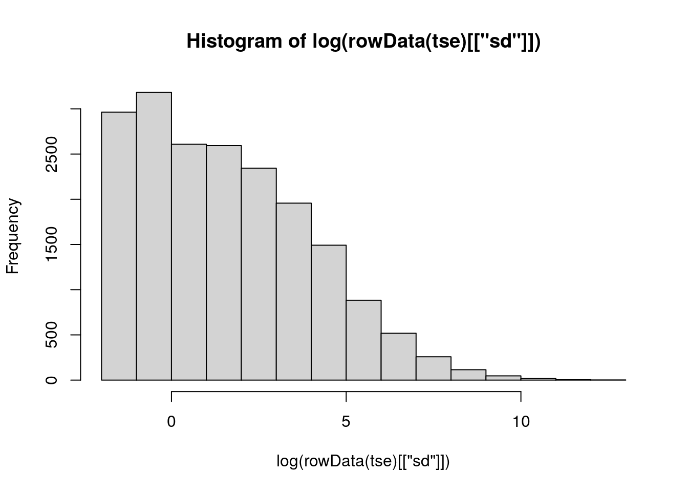
From the histogram of feature variances, we can establish a sensible threshold for filtering. For example, using a threshold of 0 would effectively remove a large set of features that show no variance.
It’s important to note that the data is on a log scale, meaning that a log-transformed value of 1 corresponds to 0 (i.e., log(1) = 0). This ensures that features with zero variance are correctly identified and filtered out.
th <- 1

selected <- rowData(tse)[["sd"]] > 1
tse_sub <- tse[selected, ]
tse_sub
##  class: TreeSummarizedExperiment
##  dim: 12840 26
##  metadata(0):
##  assays(1): counts
##  rownames(12840): 549322 522457 ... 200359 271582
##  rowData names(8): Kingdom Phylum ... Species sd
##  colnames(26): CL3 CC1 ... Even2 Even3
##  colData names(7): X.SampleID Primer ... SampleType Description
##  reducedDimNames(0):
##  mainExpName: NULL
##  altExpNames(0):
##  rowLinks: a LinkDataFrame (12840 rows)
##  rowTree: 1 phylo tree(s) (19216 leaves)
##  colLinks: NULL
##  colTree: NULL
After filtering, the dataset now contains 12840 features, compared to the original 19216 features. This means we are left with features that exhibit variance. Keep in mind that the choice of threshold depends on the specific research question, and in this case, we opted for a rather conservative threshold that retains most features.
9.6 Subset based on prevalence
We can subset the data based on prevalence using subsetByPrevalent(), which filters features that exceed a specified prevalence threshold, helping to remove rare features that may be artifacts. Conversely, subsetByRare() allows us to retain only features below the threshold, enabling a focus on rare features within the dataset.
Here, we apply a prevalence threshold of 10% and a detection threshold of 1. A feature is considered detected if it has at least one count in a sample, and prevalent if it is detected in at least 10% of the samples. The function subsetByPrevalent() retains the prevalent features, while subsetByRare() keeps the features that are not prevalent.
tse_sub <- subsetByRare(tse, rank = "Genus", prevalence = 0.1, detection = 1)
tse_sub
##  class: TreeSummarizedExperiment
##  dim: 261 26
##  metadata(1): agglomerated_by_rank
##  assays(1): counts
##  rownames(261): Acaryochloris Acetobacter ... Zooshikella p-75-a5
##  rowData names(8): Kingdom Phylum ... Species sd
##  colnames(26): CL3 CC1 ... Even2 Even3
##  colData names(7): X.SampleID Primer ... SampleType Description
##  reducedDimNames(0):
##  mainExpName: NULL
##  altExpNames(0):
##  rowLinks: a LinkDataFrame (261 rows)
##  rowTree: 1 phylo tree(s) (261 leaves)
##  colLinks: NULL
##  colTree: NULL
In some cases, agglomerating based on prevalence can provide more meaningful insights. This process is illustrated in Section 10.3.