17 Correlation
In correlation — or association analysis more generally — we can evaluate the relationships between numeric variables. These variables can be taxonomic features or patient metadata. For instance, we might be interested in which taxonomic features are present simultaneously with others, or whether body weight is associated with the abundance of certain features. In this chapter, we will demonstrate how to perform correlation analysis with mia’s getCrossAssociation() method.
17.1 Association between taxonomic features
Here we demonstrate how to analyze which bacteria co-exists in the dataset.
library(mia)

data("peerj13075")
tse <- peerj13075

# Agglomerate to certain taxonomy level
tse <- agglomerateByPrevalence(tse, rank = "class")

# Apply clr-transform and scale
tse <- transformAssay(tse, method = "clr", pseudocount = TRUE)
tse <- transformAssay(
    tse,
    assay.type = "clr", method = "standardize", MARGIN = "rows"
)

# Get correlation results
res <- getCrossAssociation(
    tse, tse,
    assay.type1 = "clr", assay.type2 = "clr",
    test.signif = TRUE, mode = "matrix"
)
We can visualize the result with a heatmap as we do later in this chapter, or we can visualize the results with a correlation network plot as done below.
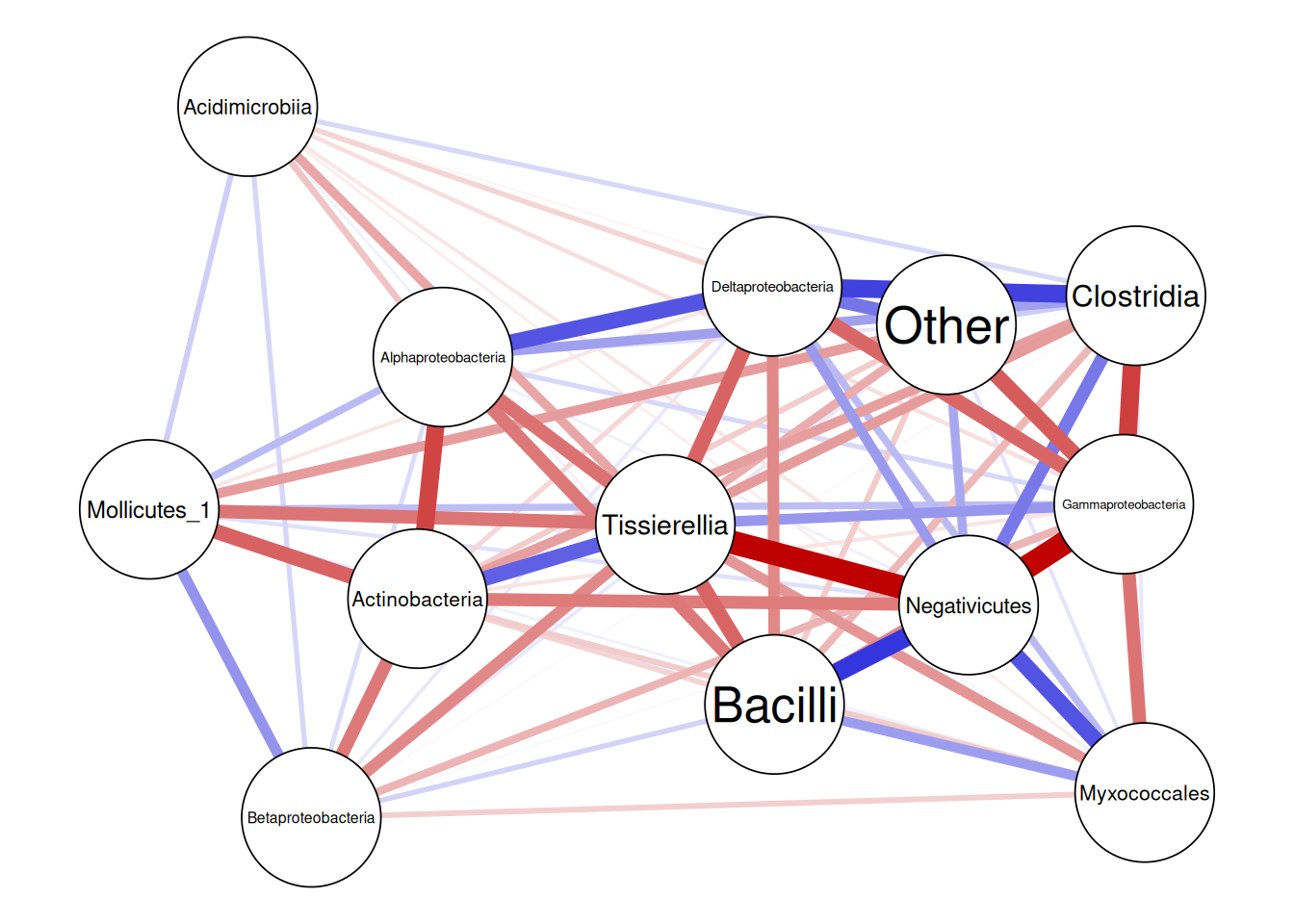
You can find more on networks from ?sec-network-learning.
17.2 Association between taxonomic features and sample metadata
Now, we can calculate alpha diversity indices, and evaluate if they have significant association with taxonomic features.
# Calculate diversity measures
index <- c(
    "shannon", "log_modulo_skewness", "coverage", "inverse_simpson", "gini"
)
tse <- addAlpha(tse, index = index)

# Get correlation results
res <- getCrossAssociation(
    tse, tse,
    assay.type1 = "clr", col.var2 = index,
    test.signif = TRUE, mode = "matrix"
)
Below, we present the results using a heatmap visualization with the help of the ComplexHeatmap and shadowtext R packages.
library(ComplexHeatmap)
library(shadowtext)

# Function for marking significant correlations with "X"
add_signif <- function(j, i, x, y, width, height, fill) {
    # If the p-value is under threshold
    if (!is.na(res$p_adj[i, j]) & res$p_adj[i, j] < 0.05) {
        # Print "X"
        grid.shadowtext(
            sprintf("%s", "X"), x, y,
            gp = gpar(fontsize = 8, col = "#f5f5f5")
        )
    }
}

# Create a heatmap
p <- Heatmap(res$cor,
    # Print values to cells
    cell_fun = add_signif,
    heatmap_legend_param = list(
        title = "correlation", legend_height = unit(5, "cm")
    ),
    column_names_rot = 45
)
p
17.3 Association between sample metadata variables
Finally, we demonstrate how to calculate correlation between sample metadata variables. Here we estimate correlation between alpha diversity measures.
Compared to the solution in Section 13.3.2.1, getCrossAssociation() allows us to calculate correlations in bulk easily, without the need for looping.
# Get correlation results
res <- getCrossAssociation(
    tse, tse,
    col.var1 = index, col.var2 = index,
    test.signif = TRUE, mode = "matrix"
)

# Create a heatmap and store it
p <- Heatmap(res$cor,
    # Print values to cells
    cell_fun = add_signif,
    heatmap_legend_param = list(
        title = "correlation", legend_height = unit(5, "cm")
    ),
    column_names_rot = 45
)
p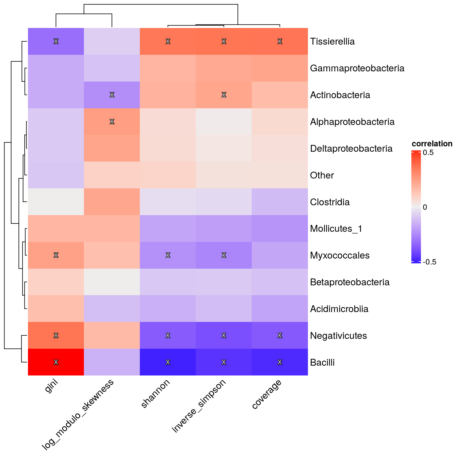
See Chapter 19 for further information on correlation and association analyses.