7 Data wrangling

This chapter introduces several essential techniques for preparing data for analysis. These techniques include splitting data, modifying data, and converting data to a data.frame. Additionally, it explains how to merge multiple SummarizedExperiment objects when needed. For a basic understanding of TreeSE please refer to Chapter 3

7.1 Splitting

You can split the data based on variables by using the functions agglomerateByRanks() and splitOn(). The former is detailed in Chapter 11.

If you want to split the data based on a variable other than taxonomic rank, use splitOn(). It works for row-wise and column-wise splitting. Splitting the data may be useful, for example, if you want to analyze data from different cohorts separately.

The following example demonstrates how to identify the most abundant taxonomic features for each sample type. Given that some samples originate from different origin, we expect differences between sample types. While getTop() can be used to determine the most abundant features across the entire dataset, this approach would obscure features that are specific to individual sample types.

library(mia)
library(knitr)

data("GlobalPatterns")
tse <- GlobalPatterns

# Agglomerate to phyla
tse <- agglomerateByRank(tse, rank = "Phylum")

# Split data based on sample type
tse_list <- splitOn(tse, by = "samples", group = "SampleType")

# Loop over the list of TreeSEs, and get top features for each
top_taxa <- sapply(tse_list, getTop)

top_taxa |> kable()

Soil	Feces	Skin	Tongue	Freshwater	Freshwater (creek)	Ocean	Sediment (estuary)	Mock
Proteobacteria	Firmicutes	Firmicutes	Proteobacteria	Cyanobacteria	Cyanobacteria	Proteobacteria	Proteobacteria	Firmicutes
Acidobacteria	Bacteroidetes	Proteobacteria	Firmicutes	Actinobacteria	Proteobacteria	Bacteroidetes	Bacteroidetes	Bacteroidetes
Verrucomicrobia	Cyanobacteria	Actinobacteria	Bacteroidetes	Proteobacteria	Bacteroidetes	Cyanobacteria	Cyanobacteria	Proteobacteria
Bacteroidetes	Actinobacteria	Bacteroidetes	Actinobacteria	Bacteroidetes	Verrucomicrobia	Actinobacteria	Crenarchaeota	Actinobacteria
Actinobacteria	Proteobacteria	Fusobacteria	Fusobacteria	Verrucomicrobia	Chloroflexi	Euryarchaeota	Planctomycetes	Tenericutes

7.2 Add or modify variables

The information contained by the colData of a TreeSE can be added and/or modified by accessing the desired variables. You might want to add or modify this data to include new variables or update existing ones, which can be essential for ensuring that all relevant metadata is available for subsequent analyses.

data("GlobalPatterns")
tse <- GlobalPatterns

# modify the Description entries
colData(tse)$Description <- paste(
    colData(tse)$Description, "modified description")

# view modified variable
tse$Description |> head()
##  [1] "Calhoun South Carolina Pine soil, pH 4.9 modified description"  
##  [2] "Cedar Creek Minnesota, grassland, pH 6.1 modified description"  
##  [3] "Sevilleta new Mexico, desert scrub, pH 8.3 modified description"
##  [4] "M3, Day 1, fecal swab, whole body study modified description"   
##  [5] "M1, Day 1, fecal swab, whole body study  modified description"  
##  [6] "M3, Day 1, right palm, whole body study modified description"

New information can be added to the experiment by creating a new variable.

# simulate new data
new_data <- runif(ncol(tse))

# store new data as new variable in colData
colData(tse)$NewVariable <- new_data

# view new variable
tse$NewVariable |> head()
##  [1] 0.3701 0.7521 0.9301 0.5453 0.7423 0.3048

Alternatively, you can add whole table by merging it with existing colData.

# simulate new data
new_data <- data.frame(var1 = runif(ncol(tse)), var2 = runif(ncol(tse)))
rownames(new_data) <- colnames(tse)

# Combine existing data with new data
colData(tse) <- cbind(colData(tse), new_data)

Similar steps can also be applied to rowData. If you have an assay whose rows and columns aling with the existing ones, you can add the assay easily to the TreeSE object.

Here we add an assay that has random numbers but in real life these steps might come handy after you have transformed the data with custom transformation that cannot be found from mia.

# Create a matrix with random values
mat <- rnorm(ncol(tse)*nrow(tse), 0, 1)
mat <- matrix(mat, ncol = ncol(tse), nrow = nrow(tse))
# Add matrix to tse
assay(tse, "random", withDimnames = FALSE) <- mat

assayNames(tse)
##  [1] "counts" "random"

Now we can see that the TreeSE object has now an additional assay called “random”. When adding new samples or features to your existing dataset, you can use cbind() to combine columns for new features or rbind() to add rows for new samples.

tse2 <- cbind(tse, tse)
tse2
##  class: TreeSummarizedExperiment 
##  dim: 19216 52 
##  metadata(0):
##  assays(2): counts random
##  rownames(19216): 549322 522457 ... 200359 271582
##  rowData names(7): Kingdom Phylum ... Genus Species
##  colnames(52): CL3 CC1 ... Even2 Even3
##  colData names(10): X.SampleID Primer ... var1 var2
##  reducedDimNames(0):
##  mainExpName: NULL
##  altExpNames(0):
##  rowLinks: a LinkDataFrame (19216 rows)
##  rowTree: 1 phylo tree(s) (19216 leaves)
##  colLinks: NULL
##  colTree: NULL

However, the aforementioned functions assume that the rows align correctly when combining columns, and vice versa. In practice, this is often not the case; for example, samples may have different feature sets. In such situations, using a merging approach is the appropriate method.

7.3 Merge data

mia package has mergeSEs() function that merges multiple SummarizedExperiment objects. For example, it is possible to combine multiple TreeSE objects which each includes one sample.

mergeSEs() works much like standard joining operations. It combines rows and columns and allows you to specify the merging method.

# Take subsets for demonstration purposes
tse1 <- tse[, 1]
tse2 <- tse[, 2]
tse3 <- tse[, 3]
tse4 <- tse[1:100, 4]

# With inner join, we want to include all shared rows. When using mergeSEs
# function all samples are always preserved.
tse <- mergeSEs(list(tse1, tse2, tse3, tse4), join = "inner")
tse
##  class: TreeSummarizedExperiment 
##  dim: 100 4 
##  metadata(0):
##  assays(1): counts
##  rownames(100): 239672 243675 ... 104332 159421
##  rowData names(7): Kingdom Phylum ... Genus Species
##  colnames(4): CC1 CL3 M31Fcsw SV1
##  colData names(10): X.SampleID Primer ... var1 var2
##  reducedDimNames(0):
##  mainExpName: NULL
##  altExpNames(0):
##  rowLinks: a LinkDataFrame (100 rows)
##  rowTree: 1 phylo tree(s) (19216 leaves)
##  colLinks: NULL
##  colTree: NULL

# Left join preserves all rows of the 1st object
tse <- mergeSEs(tse1, tse4, missing.values = 0, join = "left")
tse
##  class: TreeSummarizedExperiment 
##  dim: 19216 2 
##  metadata(0):
##  assays(1): counts
##  rownames(19216): 239672 243675 ... 239967 254851
##  rowData names(7): Kingdom Phylum ... Genus Species
##  colnames(2): CL3 M31Fcsw
##  colData names(10): X.SampleID Primer ... var1 var2
##  reducedDimNames(0):
##  mainExpName: NULL
##  altExpNames(0):
##  rowLinks: a LinkDataFrame (19216 rows)
##  rowTree: 1 phylo tree(s) (19216 leaves)
##  colLinks: NULL
##  colTree: NULL

7.4 Melting data

For several custom analysis and visualization packages, such as those from tidyverse, the SE data can be converted to a long data.frame format with meltSE().

library(knitr)

# Melt SE object
molten_tse <- meltSE(
    tse,
    assay.type = "counts",
    add.row = TRUE,
    add.col = TRUE,
    )

molten_tse |> head() |> kable()

FeatureID	SampleID	Kingdom	Phylum	Class	Order	Family	Genus	Species	X.SampleID	Primer	Final_Barcode	Barcode_truncated_plus_T	Barcode_full_length	SampleType	Description	NewVariable	var1	var2
239672	CL3	Archaea	Crenarchaeota	C2	B10	NA	NA	NA	CL3	ILBC_01	AACGCA	TGCGTT	CTAGCGTGCGT	Soil	Calhoun South Carolina Pine soil, pH 4.9 modified description	0.3701	0.9787	0.7598
239672	M31Fcsw	Archaea	Crenarchaeota	C2	B10	NA	NA	NA	M31Fcsw	ILBC_04	AAGAGA	TCTCTT	TCGACATCTCT	Feces	M3, Day 1, fecal swab, whole body study modified description	0.5453	0.6881	0.5192
243675	CL3	Archaea	Crenarchaeota	C2	B10	NA	NA	NA	CL3	ILBC_01	AACGCA	TGCGTT	CTAGCGTGCGT	Soil	Calhoun South Carolina Pine soil, pH 4.9 modified description	0.3701	0.9787	0.7598
243675	M31Fcsw	Archaea	Crenarchaeota	C2	B10	NA	NA	NA	M31Fcsw	ILBC_04	AAGAGA	TCTCTT	TCGACATCTCT	Feces	M3, Day 1, fecal swab, whole body study modified description	0.5453	0.6881	0.5192
444679	CL3	Archaea	Crenarchaeota	C2	B10	NA	NA	NA	CL3	ILBC_01	AACGCA	TGCGTT	CTAGCGTGCGT	Soil	Calhoun South Carolina Pine soil, pH 4.9 modified description	0.3701	0.9787	0.7598
444679	M31Fcsw	Archaea	Crenarchaeota	C2	B10	NA	NA	NA	M31Fcsw	ILBC_04	AAGAGA	TCTCTT	TCGACATCTCT	Feces	M3, Day 1, fecal swab, whole body study modified description	0.5453	0.6881	0.5192

For MultiAssayExperiment data, you can utilize instead longForm().

data(HintikkaXOData)
mae <- HintikkaXOData

molten_mae <- longForm(
    mae,
    i = c("counts", "nmr", "signals"),
    colDataCols = c("Rat", "Diet")
    )

molten_mae |> head() |> kable()

assay	primary	rowname	colname	value	Rat	Diet
microbiota	C1	GAYR01026362.62.2014	C1	0	1	High-fat
microbiota	C1	CVJT01000011.50.2173	C1	1	1	High-fat
microbiota	C1	KF625183.1.1786	C1	0	1	High-fat
microbiota	C1	AYSG01000002.292.2076	C1	0	1	High-fat
microbiota	C1	CCPS01000022.154.1916	C1	7	1	High-fat
microbiota	C1	KJ923794.1.1762	C1	0	1	High-fat

7.5 Tidy R programming

The tidy paradigm, first introduced in the tidyverse, promotes an intuitive and easy-to-learn coding style, which has made it popular among users. tidyomics bridges the gap between Bioconductor’s SummarizedExperiment ecosystem and the tidyverse (Hutchison et al. 2024).

Hutchison, William J., Timothy J. Keyes, Helena L. Crowell, Jacques Serizay, Charlotte Soneson, Eric S. Davis, Noriaki Sato, et al. 2024. “The Tidyomics Ecosystem: Enhancing Omic Data Analyses.” Nature Methods 21 (7): 1166–70. https://doi.org/10.1038/s41592-024-02299-2.

The package TidySingleCellExperiment can be used to manage data in TreeSE. For instance, we can easily view the object as tibble abstraction, familiar from tidyverse.

data("GlobalPatterns")
tse <- GlobalPatterns

library(tidySingleCellExperiment)

tse
##  # A SingleCellExperiment-tibble abstraction: 26 × 8
##  # [90mFeatures=19216 | Cells=26 | Assays=counts[0m
##    .cell   X.SampleID Primer  Final_Barcode Barcode_truncated_plus_T
##    <chr>   <fct>      <fct>   <fct>         <fct>                   
##  1 CL3     CL3        ILBC_01 AACGCA        TGCGTT                  
##  2 CC1     CC1        ILBC_02 AACTCG        CGAGTT                  
##  3 SV1     SV1        ILBC_03 AACTGT        ACAGTT                  
##  4 M31Fcsw M31Fcsw    ILBC_04 AAGAGA        TCTCTT                  
##  5 M11Fcsw M11Fcsw    ILBC_05 AAGCTG        CAGCTT                  
##  6 M31Plmr M31Plmr    ILBC_07 AATCGT        ACGATT                  
##  # ℹ 20 more rows
##  # ℹ 3 more variables: Barcode_full_length <fct>, SampleType <fct>, …
##  rowLinks: a LinkDataFrame (19216 rows)
##  rowTree: 1 phylo tree(s) (19216 leaves)
##  colLinks: NULL
##  colTree: NULL

By utilizing tidy programming, we could then effortlessly manipulate the data. For instance, we can calculate the mean library size in each sample type. This is done by first calculating library size for each sample and then summarizing total counts in each sample type; all done by using tidy paradigm. For more information on library size, see Chapter 9.

tse %>%
    join_features(features = rownames(tse)) %>%
    group_by(.cell) %>%
    mutate(total_counts = sum(.abundance_counts)) %>%
    group_by(SampleType) %>%
    summarise(total_counts = mean(total_counts))
##  # A tibble: 9 × 2
##    SampleType         total_counts
##    <fct>                     <dbl>
##  1 Feces                  1442116 
##  2 Freshwater             1667452 
##  3 Freshwater (creek)     1741407.
##  4 Mock                   1088484.
##  5 Ocean                  1218451 
##  6 Sediment (estuary)      277173.
##  # ℹ 3 more rows

We can then filter samples and leverage ggplot2 for plotting. In the example below, we select soil samples and visualize their abundances with a boxplot. Of course, these tidy commands can be combined with mia tools. Before plotting, we apply CLR transformation by using trasformAssay() (see more on transformation from Chapter 12).

library(ggplot2)

tse %>%
    filter(SampleType == "Soil") %>%
    transformAssay(method = "clr", pseudocount = TRUE) %>%
    join_features(features = rownames(tse)) %>%
    ggplot(aes(x = .cell, y = .abundance_clr, fill = .cell)) +
    geom_boxplot()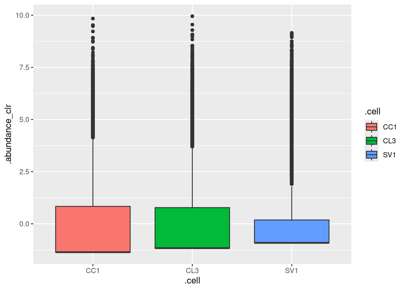

As demonstrated, tidy R programming can be effectively used to manage TreeSE objects. Please refer to tidySummarizedExperiment and tidySingleCellExperiment vignettes for more examples.

Exercises

Goal: The goal is to learn how to work with multiple datasets by merging them and splitting dataset into list of TreeSEs.

Exercise 1: Working with multiple datasets

Load any of the example datasets mentioned in Section 4.2.
Explore sample metadata.
Add arbitrary groups to colData. For instance, you create groups like this: sample(c("group1", "group2"), size = ncol(tse), replace = TRUE).
Explore the group distribution with a bar plot.
Split the data based on groups. The result should be a list containing each group in separate TreeSE.
For each TreeSE, explore the grouping variable in colData. Does each TreeSE include only one unique value?
Calculate the total number of counts in each group.
- Loop through elements of the list.
- For single TreeSE, retrieve assay, sum all the values, and add the calculated sum to colData (all the samples in certain group should have same value).
- The result should be a list of TreeSEs with additional sample metadata column.
Combine the list back to single TreeSE.
Load another dataset from Section 4.2 and merge it with the one You’ve been using. Explore the data.

Useful functions:

utils::data(), SummarizedExperiment::colData(), base::sample(), miaViz::plotBarplot(), mia::splitOn(), BiocGenerics::lapply(), SummarizedExperiment::assay(), base::sum(), mia::unsplitOn() mia::mergeSEs()