13 Alpha diversity
13.1 Background
Alpha diversity, or within-sample diversity, is a central concept in microbiome research. In ecological literature, several distinct but related alpha diversity indices, often referring to richness and evenness - the number of taxonomic features and how they are distributed, respectively - are commonly used (Willis 2019; Whittaker 1960). The term diversity can be used to collectively refer to all these indices.
13.1.1 Applications
Alpha diversity is predominantly used to quantify complexity in the microbiome. In the general adult population, lower alpha diversity and lower bacterial load have been associated with worse overall physical and mental health (Valles-Colomer et al. 2019; Vandeputte et al. 2017). However, this principle may not generalize to other populations, most notably in early life and in patient cohorts (Ma, Li, and Gotelli 2019).
13.1.2 Approaches
The majority of alpha diversity metrics are closely related, though this is not evident from their names. Bastiaanssen, Quinn, and Loughman (2023) lay out this relationship across two factors (See table below); First, alpha diversity metrics can be defined as special cases of a unifying equation of diversity, where the Hill number determines the specific index captured. Lower Hill numbers favor richness, the number of distinct taxonomic features, whereas higher numbers favor evenness, how the taxonomic features are distributed over the sample (Hill 1973). Second, some alpha diversity metrics are weighted based on phylogeny, like Faith’s PD (1992) and PhILR (Silverman et al. 2017).
Hill number 0
|
Hill number 1
|
Hill number 2
|
|
|---|---|---|---|
| Dependent on presence and absence of taxonomic features, not abundance | Dependent on how evenly taxonomic features are distributed in a sample | The probability of two randomly picked taxonomic feature not being the same | |
|
Neutral Diversity
Weighs each taxon equally, no assumptions about phylogeny |
Richness (Chao1) | Shannon Entropy | Simpson’s Index |
|
Phylogenetic Diversity
Indices are scaled based on taxonomic closeness with a phylogenetic tree |
Faith’s Phylogenetic Diversity | Phylogenetic Entropy | Rao’s Quadratic Diversity |
| The equation for general diversity can be defined as follows: ${{}^qD = (_{i=1}{R}pq_i})^{}$, with q = Hill number, R = number of features, p = relative feature abundance. | |||
Cassol, Ibañez, and Bustamante (2025) offer practical guidelines for selecting alpha diversity indices. They classify alpha diversity into four main categories and recommend calculating at least one metric from each category, if possible, to sufficiently capture within-sample diversity. Since indices within the same category tend to be correlated, they suggest using the simplest available metric. Below are the default choices for each category:
- Richness: The number of observed unique features
- Dominance: Berger-Parker
- Information: Shannon
- Phylogenetics: Faith
Several estimators have been developed to address the confounding effect of limited sampling size on observed richness, most notably ACE (A and SM 1992) and Chao1 (A 1984). Notably, these approaches may yield misleading results for modern 16S data, which commonly features denoising and removal of singletons (Deng, Umbach, and Neufeld 2024).
13.2 Rarefaction
Uneven sequencing read depth can bias diversity metrics. Rarefaction attempts to normalize read depth by repeatedly subsampling reads and computing an averaged metric(Schloss 2024a, 2024b). Rarefaction for alpha diversity metrics can be applied by specifying the optional arguments sample and niter in addAlpha(). Rarefaction is discussed in more detail in Section 14.4.2 where it is applied in the context of beta diversity.
13.3 Examples
13.3.1 Calculate alpha diversity measures
Alpha diversity can be estimated with the addAlpha() function, which includes built-in methods for calculating some indices, while others are computed via integration with the vegan package (Oksanen et al. 2020). The method calculates the given indices, and add them to the colData slot of the SummarizedExperiment object with the given name.
# First, let's load some example data.
library(mia)
data("GlobalPatterns")
tse <- GlobalPatterns

# The 'index' parameter allows computing multiple diversity indices
# simultaneously. Without specification, four standard indices are calculated:
# dbp_dominance, faith_diversity, observed_richness, and shannon_diversity.
tse <- addAlpha(
    tse,
    assay.type = "counts",
    detection = 10
)

# Check some of the first values in colData
tse$observed_richness |> head()
##  [1] 3144 3791 2319  761  671 1004
tse$shannon_diversity |> head()
##  [1] 6.577 6.777 6.498 3.828 3.288 4.289
Certain indices have additional options, here observed the detection parameter that controls the detection threshold. Species above this threshold are considered detected. See full list of options from help(addAlpha).
Because tse is a TreeSummarizedExperiment object, its phylogenetic tree is used by default. However, the optional argument tree must be provided if tse does not contain a rowTree.
13.3.2 Visualize alpha diversity measures
As alpha diversity metrics typically summarize high-dimensional samples into singular values, many visualization approaches are available. Once calculated, these metrics can be analyzed directly from the colData, for example, by plotting them using plotColData() from the scater package (McCarthy et al. 2020). Here, we use the observed species as a measure of richness. Let’s visualize the results against selected colData variables (sample type and final barcode).
library(scater)
plotColData(
    tse,
    "observed_richness",
    "SampleType",
    colour_by = "Final_Barcode"
) +
    theme(axis.text.x = element_text(angle = 45, hjust = 1)) +
    labs(x = "Sample types", y = expression(Richness[observed_richness]))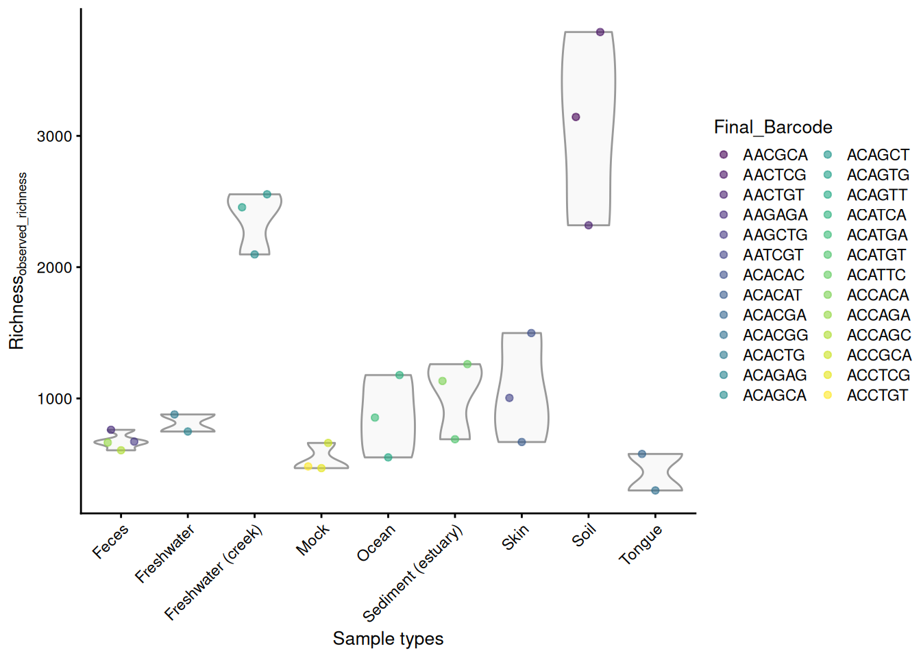
13.3.2.1 Alpha diversity measures comparisons
We can compare alpha diversities for example by calculating the correlation between them. Below, a visual comparison between Shannon and Faith indices is shown with a scatter plot.
plotColData(tse, x = "shannon_diversity", y = "faith_diversity") +
    labs(x = "Shannon index", y = "Faith (phylogenetic) index") +
    geom_smooth(method = "lm")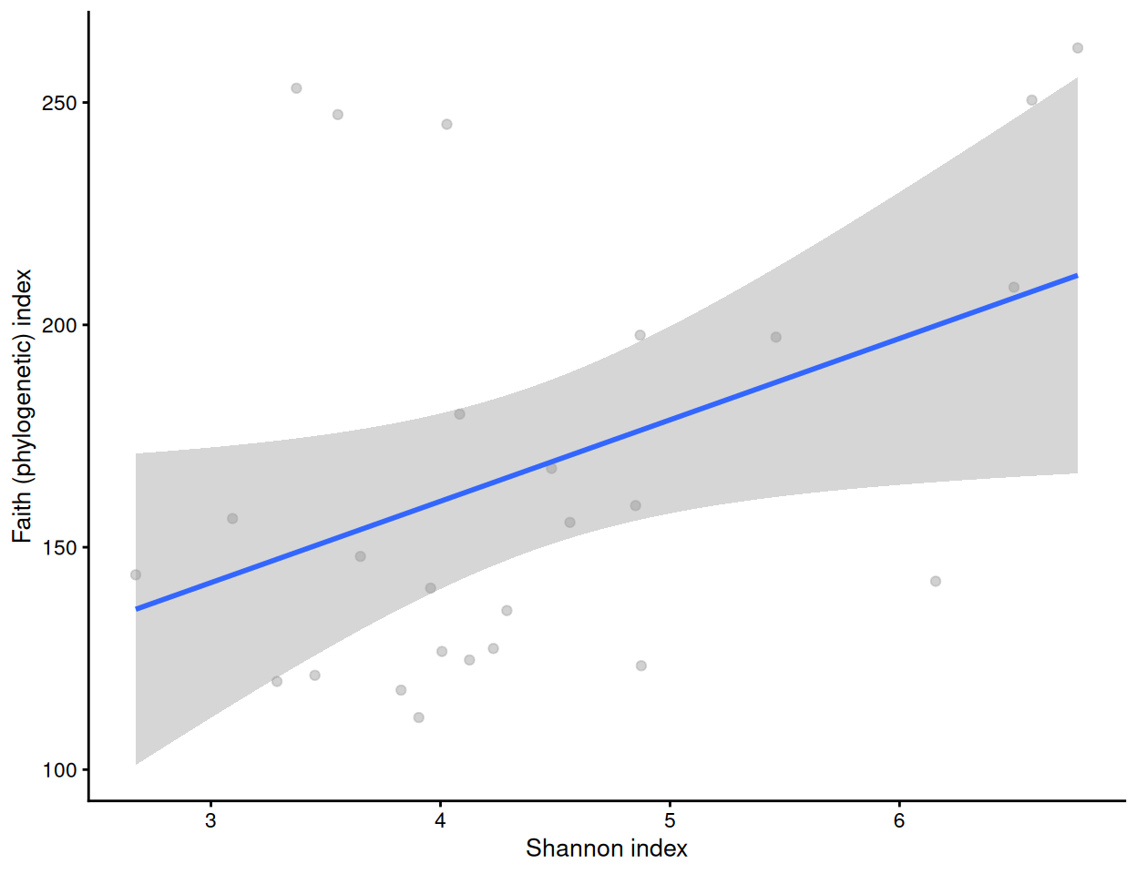
cor.test(tse[["shannon_diversity"]], tse[["faith_diversity"]])
##
##      Pearson's product-moment correlation
##
##  data:  tse[["shannon_diversity"]] and tse[["faith_diversity"]]
##  t = 2.2, df = 24, p-value = 0.04
##  alternative hypothesis: true correlation is not equal to 0
##  95 percent confidence interval:
##   0.02719 0.68822
##  sample estimates:
##     cor
##  0.4102
Let us visualize results from multiple alpha diversity measures against a given sample grouping available in colData (here, sample type). These have been readily stored in the colData slot, and they are thus directly available for plotting.
library(patchwork)

# Create the plots
indices <- c(
    "observed_richness", "dbp_dominance", "shannon_diversity",
    "faith_diversity"
)
plots <- lapply(
    indices,
    plotColData,
    object = tse,
    x = "SampleType",
    colour_by = "SampleType"
)

# Fine-tune visual appearance
plots <- lapply(
    plots, "+",
    theme(
        axis.text.x = element_blank(),
        axis.title.x = element_blank(),
        axis.ticks.x = element_blank()
    )
)

# Plot the figures
wrap_plots(plots, ncol = 1) +
    plot_layout(guides = "collect")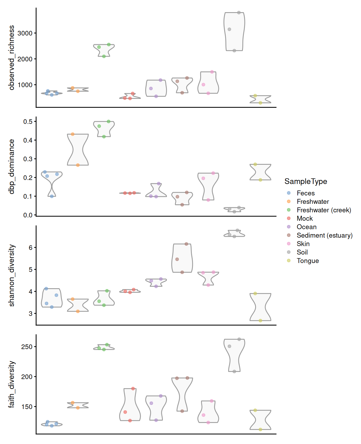
All these different metrics provide information from different aspects of alpha diversity, notably on richness, dominance, information, and phylogenetic diversity described in Cassol, Ibañez, and Bustamante (2025). It is recommended to interpret these aspects separately and together.
From our example, we can observe that soil and freshwater (creek) have the highest number of different taxonomic features present while tongue microbiome has the lowest richness, suggesting greater biodiversity in soil and freshwater samples.
Based on the dominance values, species abundances in the soil samples appeared to be relatively evenly distributed. In contrast, the freshwater microbiome — particularly in the freshwater creek samples — was dominated by a single species, despite showing high observed richness.
These observations are supported by the Shannon index, which accounts for both richness and dominance. Soil samples showed the highest Shannon diversity, reflecting their high number of observed species and relatively even species distribution.
Soil and freshwater creek environments host a wide range of phylogenetically diverse organisms, indicating that the observed taxonomic features are not closely related but rather distinct from one another in terms of their evolutionary history.
In summary, soil samples exhibit the highest biodiversity, while human-derived samples show less variation in terms of species composition and evolutionary diversity.
13.3.3 Statistical analysis of alpha diversity measures
We can then analyze the statistical significance. We use the non-parametric Wilcoxon or Mann-Whitney test, as it is more flexible than the commonly used Student’s t-Test, since it does not assume normality.
pairwise.wilcox.test(
    tse[["observed_richness"]], tse[["SampleType"]],
    p.adjust.method = "fdr"
)
##
##      Pairwise comparisons using Wilcoxon rank sum exact test
##
##  data:  tse[["observed_richness"]] and tse[["SampleType"]]
##
##                     Feces Freshwater Freshwater (creek) Mock Ocean
##  Freshwater         0.4   -          -                  -    -
##  Freshwater (creek) 0.3   0.3        -                  -    -
##  Mock               0.3   0.3        0.3                -    -
##  Ocean              0.8   1.0        0.3                0.3  -
##  Sediment (estuary) 0.3   0.8        0.3                0.3  0.8
##  Skin               0.3   0.8        0.3                0.3  0.8
##  Soil               0.3   0.3        0.5                0.3  0.3
##  Tongue             0.3   0.5        0.3                0.8  0.5
##                     Sediment (estuary) Skin Soil
##  Freshwater         -                  -    -
##  Freshwater (creek) -                  -    -
##  Mock               -                  -    -
##  Ocean              -                  -    -
##  Sediment (estuary) -                  -    -
##  Skin               1.0                -    -
##  Soil               0.3                0.3  -
##  Tongue             0.3                0.3  0.3
##
##  P value adjustment method: fdr
13.3.3.1 Visualizing significance in group-wise comparisons
Next, let’s compare the Shannon index between sample groups and visualize the statistical significance. Using the stat_compare_means function from the ggpubr package, we can add visually appealing p-values to our plots.
To add adjusted p-values, we first have to calculate them.
library(ggpubr)
library(tidyverse)


index <- "shannon_diversity"
group_var <- "SampleType"

# Subsets the data by selecting only samples from feces, skin, or tongue.
tse_sub <- tse[, tse[[group_var]] %in% c("Feces", "Skin", "Tongue")]

# Updates factor levels to reflect selected groups
tse_sub$SampleType <- factor(tse_sub$SampleType)

# Calculate p-values
pvals <- pairwise.wilcox.test(
    tse_sub[[index]], tse_sub[[group_var]],
    p.adjust.method = "fdr"
)

# Put them to data.frame format
pvals <- pvals[["p.value"]] |>
    as.data.frame()
varname <- "group1"
pvals[[varname]] <- rownames(pvals)

# To long format
pvals <- reshape(
    pvals,
    direction = "long",
    varying = colnames(pvals)[!colnames(pvals) %in% varname],
    times = colnames(pvals)[!colnames(pvals) %in% varname],
    v.names = "p",
    timevar = "group2",
    idvar = "group1"
) |>
    na.omit()

# Add y-axis position
pvals[["y.position"]] <- apply(pvals, 1, function(x) {
    temp1 <- tse[[index]][tse[[group_var]] == x[["group1"]]]
    temp2 <- tse[[index]][tse[[group_var]] == x[["group2"]]]
    temp <- max(c(temp1, temp2))
    return(temp)
})
pvals[["y.position"]] <- max(pvals[["y.position"]]) +
    order(pvals[["y.position"]]) * 0.2

# Round values
pvals[["p"]] <- round(pvals[["p"]], 3)

# Create a boxplot
p <- plotColData(
    tse_sub,
    x = group_var, y = index,
    show_boxplot = TRUE, show_violin = FALSE
) +
    theme(text = element_text(size = 10)) +
    stat_pvalue_manual(pvals)
p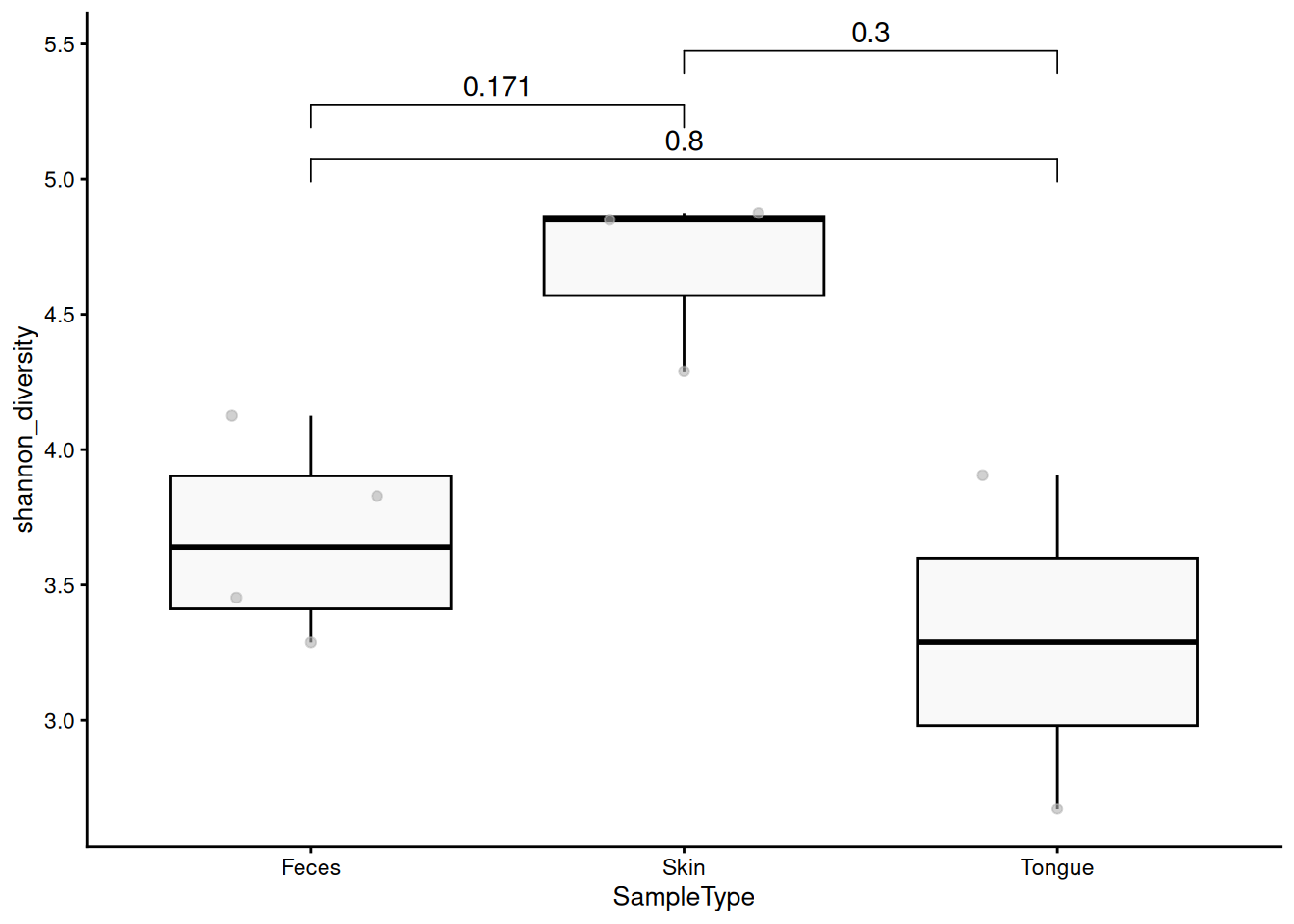
13.4 Further reading
An article on ggpubr package provides further examples for estimating and highlighting significances.