Supervised methods

Estimated time: 85 minutes

Overview

Questions

• Can we predict an outcome from several data types together?
• Which data types and which features predict the outcome?
• What are early, intermediate and late fusion?

Objectives

• Explain early, intermediate and late fusion (stacking) of several data types.
• Train a multi-omics prediction model with IntegratedLearner and evaluate it with cross-validation.
• Interpret the weights that IntegratedLearner gives to each data type.
• Explain the idea of sparse partial least squares, and find the features of several data types that together tell the groups apart with DIABLO.
• Describe what IntegratedLearner and DIABLO show about the data.

Where are we?

---

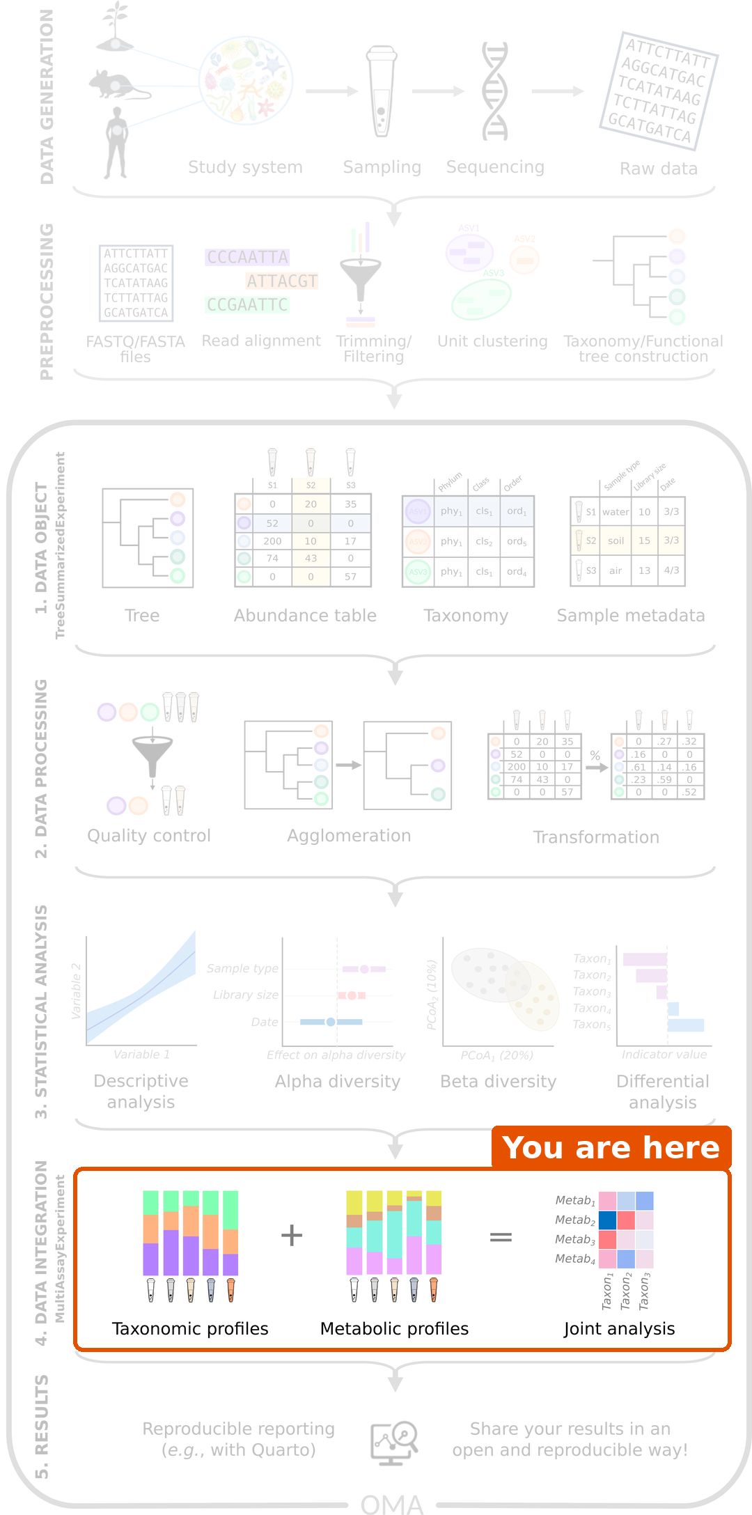
In the previous episode, the unsupervised methods found the main pattern that the data types share: the fat in the diet. They did not find the effect of XOS, because it is smaller.

Supervised methods are given an outcome, such as the diet group, and look for the features that predict it. Machine learning on a single microbiome table can predict, for example, a disease. Now we predict from several data types.

Method	What it gives
IntegratedLearner	A prediction from all data types, how well it works, and how much each data type contributes
DIABLO	The features of each data type that together tell the groups apart

Load packages

---

R

library(mia)
library(MultiAssayExperiment)
library(IntegratedLearner)
library(mixOmics)

We continue with the mae object that we prepared in episode 2.

Three ways to combine data types

---

How do we feed several tables to one prediction model? There are three common strategies, called fusion:

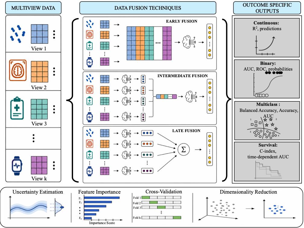
Figure: IntegratedLearner (MIT licence).

• Early fusion: join all tables side by side into one big table, and train one model on it. This is simple, but the largest table (here the microbiota) can dominate the model.
• Intermediate fusion: train a model on each table, join what the models learned, and train one more model on top.
• Late fusion: train a separate model on each table, and combine their predictions, for example as a weighted average. The weights tell how much each data type contributes. Combining predictions with a second model is called stacking.

IntegratedLearner

---

IntegratedLearner (Mallick et al. 2024) fits both early fusion (the concatenated model) and late fusion (the stacked model), and compares them with the models of the single data types. It can use many machine learning methods as base learners, the models of the single data types; we use random forest.

How does stacking work? Each base learner predicts every rat with cross-validation, so each rat gets one predicted probability per data type from models that did not see it. A meta-learner then learns how to combine these probabilities. By default, it finds non-negative weights that sum to 1 and give the best AUC. A data type that predicts well gets a large weight, and a data type that adds nothing gets a weight near 0.

Prepare the data

IntegratedLearner reads the outcome and the sample IDs from the sample information of each experiment, not from the shared colData() of the MAE. getWithColData() adds the sample information to an experiment, as in episode 2. We do this for each of the three experiments:

R

mae[["microbiota"]] <- getWithColData(mae, "microbiota")
mae[["metabolites"]] <- getWithColData(mae, "metabolites")
mae[["biomarkers"]] <- getWithColData(mae, "biomarkers")
colnames(colData(mae[["metabolites"]]))

OUTPUT

[1] "Sample" "Rat"    "Site"   "Diet"   "Fat"    "XOS"   

Train the model

We predict whether a rat was fed the high-fat diet (Fat). The arguments are:

• experiment and assay.type: the data types and the table to use from each. Random forest works directly on the counts of the microbiota.
• outcome_col and subject_id_col: the columns of the sample information with the outcome and the rat.
• na.rm = TRUE: drop the features with missing values (some biomarkers).
• folds = 5: evaluate the models with 5-fold cross-validation.
• base_learner: the machine learning method, here random forest.
• family = binomial(): the outcome has two classes.
• seed: fixes the random split into folds. The random forests are random too, so we also run set.seed() first.

R

set.seed(123)
fit <- IntegratedLearner(
    MAE_train = mae,
    experiment = c("microbiota", "metabolites", "biomarkers"),
    assay.type = c("counts", "log10", "signals"),
    outcome_col = "Fat",
    subject_id_col = "Sample",
    na.rm = TRUE,
    folds = 5,
    base_learner = "SL.randomForest",
    family = binomial(),
    seed = 123
)

OUTPUT

Time for model fit : 0.027 minutes
========================================
Model fit for individual layers: SL.randomForest
Model fit for stacked layer: sl_nnls_auc
Model fit for concatenated layer: SL.randomForest
========================================
AUC metric for training data:
Individual layers:
 biomarkers metabolites  microbiota
      1.000       1.000       0.968
======================
Stacked model:1
======================
Concatenated model:1
======================
========================================
Weights for individual layers predictions in IntegratedLearner:
 biomarkers metabolites  microbiota
      0.579       0.016       0.405
========================================

The summary shows the AUC of each model. The printout calls it “training data”, but the AUCs are calculated from the cross-validated predictions: each rat is predicted by a model that did not see it during training, as with a separate test set.

How good are the predictions?

fit$metrics.train collects the AUC, accuracy and balanced accuracy of each model:

R

fit$metrics.train

OUTPUT

         model   auc accuracy balanced_accuracy
1   biomarkers 1.000      1.0               1.0
2  metabolites 1.000      1.0               1.0
3   microbiota 0.968      0.9               0.9
4      stacked 1.000      1.0               1.0
5 concatenated 1.000      1.0               1.0

plot() draws the ROC curve of each model. It returns the plot and a table of the curves; we show only the plot:

R

plot(fit)$plot

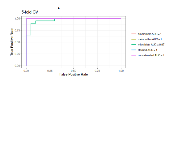
Result: every model predicts the fat in the diet very well (cross-validated AUC from 0.968 to 1). The fat has such a large effect that any one data type is enough to predict it.

How much does each data type contribute?

The late fusion (stacked) model combines the predictions of the three data types with weights:

R

fit$weights

OUTPUT

 biomarkers metabolites  microbiota
 0.57877869  0.01623401  0.40498730 

Result: the stacked model relies most on the biomarkers (weight 0.58). But when all data types predict equally well, as here, any of them will do, and the weights change a lot with the random seed. Interpret the weights only when the data types differ in how well they predict.

Challenge

Challenge 1 (about 20 minutes): Can we predict XOS?

The unsupervised methods could not find the effect of XOS. Can a supervised method predict it?

1. Train an IntegratedLearner model that predicts XOS instead of Fat, with the same settings otherwise.
2. Look at the AUC of each model. Which data type predicts XOS best? How well does it work compared with predicting the fat?
3. Look at the weights of the stacked model. Which data types does it use?
4. Does combining the data types improve the prediction over the best single data type?

Show me the solution

R

set.seed(123)
fit_xos <- IntegratedLearner(
    MAE_train = mae,
    experiment = c("microbiota", "metabolites", "biomarkers"),
    assay.type = c("counts", "log10", "signals"),
    outcome_col = "XOS",
    subject_id_col = "Sample",
    na.rm = TRUE,
    folds = 5,
    base_learner = "SL.randomForest",
    family = binomial(),
    seed = 123
)

OUTPUT

Time for model fit : 0.023 minutes
========================================
Model fit for individual layers: SL.randomForest
Model fit for stacked layer: sl_nnls_auc
Model fit for concatenated layer: SL.randomForest
========================================
AUC metric for training data:
Individual layers:
 biomarkers metabolites  microbiota
      0.575       0.609       0.425
======================
Stacked model:0.565
======================
Concatenated model:0.531
======================
========================================
Weights for individual layers predictions in IntegratedLearner:
 biomarkers metabolites  microbiota
      0.526       0.405       0.069
========================================

R

fit_xos$metrics.train

OUTPUT

         model   auc accuracy balanced_accuracy
1   biomarkers 0.575    0.575             0.575
2  metabolites 0.609    0.550             0.550
3   microbiota 0.425    0.425             0.425
4      stacked 0.565    0.575             0.575
5 concatenated 0.531    0.500             0.500

R

fit_xos$weights

OUTPUT

 biomarkers metabolites  microbiota
 0.52577398  0.40494153  0.06928449 

XOS is much harder to predict than the fat. The best single data type is the metabolites (AUC 0.609). The stacked model has an AUC of 0.565 and the concatenated model 0.531.

Neither combined model is better than the best single data type. Combining the data types does not create a signal that is not in the data. With only 40 rats and a small effect, the predictions are uncertain: with another random seed, the numbers change. An AUC around 0.6 is only a little better than guessing (0.5).

Callout

More in IntegratedLearner

• base_learner = "sl_bart" (the default) uses Bayesian additive regression trees, which also give the uncertainty of the predictions and of the feature importance. It needs Java and takes longer to run.
• run_intermediate = TRUE fits an intermediate fusion model (cooperative learning).
• MAE_valid takes an independent validation dataset.

See the IntegratedLearner documentation and the OMA chapter on machine learning.

DIABLO

---

IntegratedLearner tells us how well the data types predict the outcome. DIABLO (Singh et al. 2019), from the mixOmics package, focuses on which features do it. It looks for a few components (like PCA axes) that

• separate the groups, and
• are correlated between the data types,

and it selects a small number of features from each data type for each component.

DIABLO is based on sparse partial least squares (sPLS). A PCA finds the direction in one table along which the samples vary most. PLS instead finds one direction in each table, chosen so that the sample scores along the directions are as correlated as possible, between the tables and with the outcome. Sparse means that only a few features get a non-zero weight; the others are set to 0. The selected features form a short signature.

Prepare the data

mixOmics does not read a MAE. It takes a list of matrices with the samples as rows, so we transpose the tables with t(). We use the rclr values of the microbiota and the log10 values of the metabolites:

R

X <- list(
    microbiota = t(assay(mae[["microbiota"]], "rclr")),
    metabolites = t(assay(mae[["metabolites"]], "log10"))
)
Y <- mae$Fat
identical(rownames(X$microbiota), rownames(X$metabolites))

OUTPUT

[1] TRUE

R

identical(rownames(X$microbiota), rownames(colData(mae)))

OUTPUT

[1] TRUE

The rows of both matrices and the outcome must be in the same order; the two checks confirm it. We leave out the biomarkers, which have missing values. DIABLO standardizes each feature itself (scale = TRUE).

Train the model

DIABLO needs the number of components (ncomp) and the number of features to select from each data type for each component (keepX). Here we select 10 genera and 5 metabolites for each of 2 components:

R

diablo <- block.splsda(
    X, Y, ncomp = 2,
    keepX = list(microbiota = c(10, 10), metabolites = c(5, 5))
)

The design argument sets how strongly the components of the data types should be correlated with each other, from 0 to 1. By default, it is 1: DIABLO looks for components that are as correlated as possible between the data types. A smaller value, such as 0.1, puts more weight on separating the groups.

Plot the samples

plotIndiv() draws the samples on the first two components, once for each data type:

R

plotIndiv(diablo, legend = TRUE, title = "DIABLO")

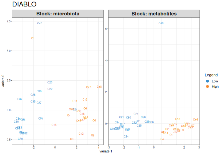
Result: in both data types, the first component clearly separates the high-fat and the low-fat rats.

How good is it?

The separation in the plot is on the same data that the model was trained on. As always in machine learning, we estimate the error with cross-validation. perf() repeats a 5-fold cross-validation 10 times. The folds are random, so we fix them with the seed argument:

R

perf_diablo <- perf(diablo, validation = "Mfold", folds = 5, nrepeat = 10,
                    seed = 123)
perf_diablo$WeightedVote.error.rate$centroids.dist

OUTPUT

             comp1 comp2
Low         0.0700 0.065
High        0.0050 0.005
Overall.ER  0.0375 0.035
Overall.BER 0.0375 0.035

The table shows the error rate for each group and overall (Overall.ER), with one and with two components.

Result: with one component, 4 % of the rats are classified wrongly, and with two components 4 %.

Which features tell the groups apart?

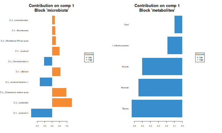
plotLoadings() shows the features selected for a component and their weights. contrib = "max" colours each feature by the group in which it is highest:

R

plotLoadings(diablo, comp = 1, contrib = "max", method = "median")

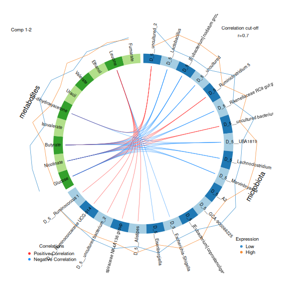
circosPlot() draws the correlations between the selected features of the two data types. Lines connect features with a correlation above cutoff:

R

circosPlot(diablo, cutoff = 0.7, line = TRUE, size.labels = 1.2,
           size.variables = 0.7)

The selected features of component 1 are also listed by selectVar():

R

selectVar(diablo, comp = 1)$metabolites$name

OUTPUT

[1] "Glucose"              "Nicotinate"           "Butyrate"
[4] "1,3-dihydroxyacetone" "Uracil"              

Result: the metabolites that tell the diets apart on component 1 are Glucose, Nicotinate, Butyrate, 1,3-dihydroxyacetone, Uracil. The circos plot shows that several of them are strongly correlated with the selected genera, both positively and negatively.

Challenge

Challenge 2: Compare the methods

1. Compare the metabolites selected by DIABLO with the metabolites that MiRKAT found in episode 3, and those with the largest weights on MOFA factor 1 in episode 4. Which metabolites appear in all of them?
2. What does each method tell you that the others do not?

Show me the solution

1. All five metabolites that DIABLO selected are also significant in MiRKAT and among the ten largest weights of MOFA factor 1. Glucose, butyrate and nicotinate are at the top of all three lists. Metabolites that are found by methods that work in different ways are good candidates for follow-up.

2. MiRKAT tells which metabolites are related to the microbiota as a whole. MOFA tells which features drive the main shared pattern, without knowing the groups. DIABLO selects the features that together tell the groups apart and are correlated between the data types. IntegratedLearner tells how well the data types predict the outcome, and how much each of them contributes.

Challenge

Challenge 3 (about 15 minutes): DIABLO for XOS

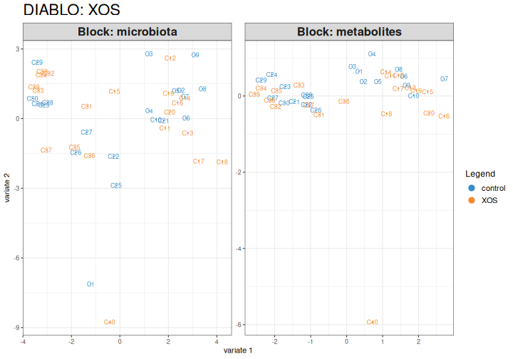
1. Train a DIABLO model that predicts XOS, with the same settings.
2. Draw the samples with plotIndiv(). Are the groups separated?
3. Estimate the error with perf(). Compare it with the model for the fat.
4. Draw the samples again, but colour them by fat (group = mae$Fat). What does the first component separate?

Show me the solution

R

diablo_xos <- block.splsda(
    X, mae$XOS, ncomp = 2,
    keepX = list(microbiota = c(10, 10), metabolites = c(5, 5))
)
plotIndiv(diablo_xos, legend = TRUE, title = "DIABLO: XOS")

R

perf_xos <- perf(diablo_xos, validation = "Mfold", folds = 5, nrepeat = 10,
                 seed = 123)
perf_xos$WeightedVote.error.rate$centroids.dist

OUTPUT

            comp1  comp2
control      0.58 0.5000
XOS          0.56 0.5250
Overall.ER   0.57 0.5125
Overall.BER  0.57 0.5125

The groups overlap more than for the fat, even on the training data. The cross-validated error is about 51 %, compared with 4 % for the fat. With two equally large groups, guessing gives an error of 50 %. DIABLO always finds some separation on the training data, because it is built to do so. This is why the cross-validated error is the number to report.

R

plotIndiv(diablo_xos, group = mae$Fat, legend = TRUE,
          title = "DIABLO: XOS, coloured by fat")

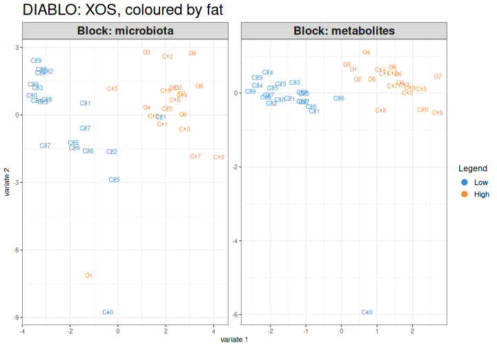
The first component of the XOS model largely separates the high-fat and the low-fat rats. DIABLO also looks for components that are correlated between the data types, and the strongest shared pattern is the fat. The design argument (for example design = 0.1) gives more weight to the outcome.

Two views of the same question

---

IntegratedLearner and DIABLO are both supervised, but they show different things:

• IntegratedLearner tells how well the data types predict the outcome, alone and combined, and how much each data type contributes. It can use many machine learning methods, and outcomes of many kinds.
• DIABLO selects a few features from each data type that together tell the groups apart and are correlated with each other.

In our data, both find that the fat is easy to predict and XOS is not. Whatever the method, evaluate the model with cross-validation or an independent dataset.

Callout

Learn more

Choose ncomp and keepX with perf() and tune.block.splsda(), and set how strongly the data types should be correlated with the design argument. See the DIABLO tutorial and the OMA chapter on multi-omics.

References

---

• Mallick H. et al. (2024) An integrated Bayesian framework for multi-omics prediction and classification. Statistics in Medicine 43: 983–1002.
• Singh A. et al. (2019) DIABLO: an integrative approach for identifying key molecular drivers from multi-omics assays. Bioinformatics 35: 3055–3062.

Key Points

• Supervised integration predicts an outcome from several data types. Early fusion joins the tables, late fusion combines the predictions of separate models, and intermediate fusion combines what separate models learned.
• IntegratedLearner() trains models on a MultiAssayExperiment and reports cross-validated AUCs for each data type and for early and late fusion, plus the weight of each data type.
• DIABLO (block.splsda()) selects a few features from each data type that together tell the groups apart and are correlated with each other.
• Always evaluate a supervised model with cross-validation. Combining data types does not create a signal that is not in the data.