Authors: Axel Dagnaud, Noah de Gunst, Tuomas Borman, Leo Lahti.
Version: 2.1
Last modified: 1 September, 2024.
 French
  Dutch
Dutch ![]()
Introduction
Hello and welcome to a comprehensive workflow using the latest R/Bioconductor tools for microbiome data science. In this tutorial, we’ll guide you through the foundational steps of microbiome analysis using miaverse. These steps are applicable to almost any of your projects and will help you understand the fundamental concepts that will skyrocket 🚀 your future microbiome analyses.
In this workflow, we cover basics of:
- Data wrangling and transformations
- Exploration
- Alpha and beta diversity
Load packages
To begin, we need to load the necessary packages. The following script ensures that all required packages are loaded and installed if they aren’t already.
# List of packages that we need
packages <- c("mia",  "miaViz", "scater")

# Get packages that are already installed
packages_already_installed <- packages[ packages %in% installed.packages() ]

# Get packages that need to be installed
packages_need_to_install <- setdiff( packages, packages_already_installed )

# Loads BiocManager into the session. Install it if it is not already installed.
if( !require("BiocManager") ){
    install.packages("BiocManager")
    library("BiocManager")
}

# If there are packages that need to be installed, installs them with
# BiocManager
if( length(packages_need_to_install) > 0 ) {
   install(packages_need_to_install, ask = FALSE)
}

# Load all packages into session. Stop if there are packages that were not
# successfully loaded
pkgs_not_loaded <- !sapply(packages, require, character.only = TRUE)
pkgs_not_loaded <- names(pkgs_not_loaded)[ pkgs_not_loaded ]
if( length(pkgs_not_loaded) > 0 ){
    stop(
        "Error in loading the following packages into the session: '",
        paste0(pkgs_not_loaded, collapse = "', '"), "'")
}
Importing data
The next step involves importing your data into the R environment.
Depending on the bioinformatics tools used in the upstream section of
the workflow, importing the data may vary slightly. We cover the most
widely used formats, with importers available for convenience. You can
also build a TreeSummarizedExperiment (TreeSE)
from scratch from basic text files. For more information, see OMA.
For this demonstration, you can either use your own data or one of the built-in datasets provided by mia, which you can find here.
In this tutorial, we’ll be using the @Tengeler2020 dataset. In the study, they explored the impact of altered microbiomes on brain structure, specifically comparing patients with ADHD (Attention Deficit Hyperactivity Disorder) to controls (see more information on this dataset from here). Let’s load this dataset into our R environment:
data("Tengeler2020", package = "mia")
tse <- Tengeler2020
Subsetting and accessing the data
Once loaded, we often need to wrangle and preprocess the data. The
TreeSE object, a primary data container in the
miaverse framework, is designed to handle complex microbiome
data effectively. For more details about the TreeSE and
other data containers, see OMA.
Subsetting
In many cases, you may need to work with only a portion of your
original TreeSE for various reasons. Subsetting the
TreeSE object is as straightforward as manipulating a basic
matrix in R, utilizing rows and columns. For example, using the
Tengeler2020 dataset, we can focus on a specific cohort. Here’s how:
dim(tse)
#> [1] 151  27
# Subset based on sample metadata
tse <- tse[ , tse$cohort == "Cohort_2" ]
dim(tse)
#> [1] 151  10
This will create a TreeSE object only containing samples
of the second cohort. You can find more information on subsetting from
here.
Accessing data
You can also access different types of data stored within the
TreeSE object. Here’s a quick reminder on how to access
certain types of data:
You can access the abundance table, or assays, as follows. In this example, we specify that we want to fetch an abundance table named “counts”. For more details, see OMA.
assay(tse, "counts") |> head()
#>                  A21  A23  A25  A28 A29 A210  A22  A24  A26  A27
#> Bacteroides     1740 1791 2368 1316 252 4052 1838 3085 1570 3621
#> Bacteroides_1    540  229    0    0   0 1762    0 2190    0 1480
#> Parabacteroides  145    0  109  119  31    0 5415    0 3531    0
#> Bacteroides_2    659    0  588  542 141    0  796   84  135  293
#> Akkermansia       84  700  440  244  25 2456  976  316 2420 1129
#> Bacteroides_3    610    0  522  511 352    0    0   70    0  322
Sample (or column) metadata is stored in colData. In
this example, it includes the diagnoses of the patients from whom the
samples were drawn.
colData(tse)
#> DataFrame with 10 rows and 4 columns
#>      patient_status      cohort patient_status_vs_cohort sample_name
#>         <character> <character>              <character> <character>
#> A21            ADHD    Cohort_2            ADHD_Cohort_2         A21
#> A23            ADHD    Cohort_2            ADHD_Cohort_2         A23
#> A25            ADHD    Cohort_2            ADHD_Cohort_2         A25
#> A28            ADHD    Cohort_2            ADHD_Cohort_2         A28
#> A29            ADHD    Cohort_2            ADHD_Cohort_2         A29
#> A210        Control    Cohort_2         Control_Cohort_2        A210
#> A22         Control    Cohort_2         Control_Cohort_2         A22
#> A24         Control    Cohort_2         Control_Cohort_2         A24
#> A26         Control    Cohort_2         Control_Cohort_2         A26
#> A27         Control    Cohort_2         Control_Cohort_2         A27
rowData contains data on feature characteristics,
particularly taxonomic information.
rd <- rowData(tse)
rd
#> DataFrame with 151 rows and 6 columns
#>                                      Kingdom          Phylum
#>                                  <character>     <character>
#> Bacteroides                         Bacteria   Bacteroidetes
#> Bacteroides_1                       Bacteria   Bacteroidetes
#> Parabacteroides                     Bacteria   Bacteroidetes
#> Bacteroides_2                       Bacteria   Bacteroidetes
#> Akkermansia                         Bacteria Verrucomicrobia
#> ...                                      ...             ...
#> Unidentified_Gastranaerophilales    Bacteria   Cyanobacteria
#> Halomonas                           Bacteria  Proteobacteria
#> Lachnoclostridium_4                 Bacteria      Firmicutes
#> Parabacteroides_8                   Bacteria   Bacteroidetes
#> Unidentified_Lachnospiraceae_14     Bacteria      Firmicutes
#>                                                Class               Order
#>                                          <character>         <character>
#> Bacteroides                              Bacteroidia       Bacteroidales
#> Bacteroides_1                            Bacteroidia       Bacteroidales
#> Parabacteroides                          Bacteroidia       Bacteroidales
#> Bacteroides_2                            Bacteroidia       Bacteroidales
#> Akkermansia                         Verrucomicrobiae  Verrucomicrobiales
#> ...                                              ...                 ...
#> Unidentified_Gastranaerophilales     Melainabacteria Gastranaerophilales
#> Halomonas                        Gammaproteobacteria   Oceanospirillales
#> Lachnoclostridium_4                       Clostridia       Clostridiales
#> Parabacteroides_8                        Bacteroidia       Bacteroidales
#> Unidentified_Lachnospiraceae_14           Clostridia       Clostridiales
#>                                               Family             Genus
#>                                          <character>       <character>
#> Bacteroides                           Bacteroidaceae       Bacteroides
#> Bacteroides_1                         Bacteroidaceae       Bacteroides
#> Parabacteroides                   Porphyromonadaceae   Parabacteroides
#> Bacteroides_2                         Bacteroidaceae       Bacteroides
#> Akkermansia                      Verrucomicrobiaceae       Akkermansia
#> ...                                              ...               ...
#> Unidentified_Gastranaerophilales
#> Halomonas                             Halomonadaceae         Halomonas
#> Lachnoclostridium_4                  Lachnospiraceae Lachnoclostridium
#> Parabacteroides_8                 Porphyromonadaceae   Parabacteroides
#> Unidentified_Lachnospiraceae_14      Lachnospiraceae        uncultured
Here rowData(tse) returns a DataFrame with 151 rows and
7 columns. Each row represents an organism and each column a taxonomic
level.
Data wrangling
Agglomerating data
Agglomerating your data to a specific taxonomic rank helps simplify
the analysis and reveal broader patterns. By grouping taxonomic features
at a chosen level, such as Phylum, you can better understand general
trends and distributions. The agglomerateByRank() function
streamlines this process, making it easier to analyze and visualize data
at a higher level of aggregation.
tse_phylum <- agglomerateByRank(tse, rank = "Phylum")

# Check
tse_phylum
#> class: TreeSummarizedExperiment
#> dim: 5 10
#> metadata(1): agglomerated_by_rank
#> assays(1): counts
#> rownames(5): Bacteroidetes Cyanobacteria Firmicutes Proteobacteria
#>   Verrucomicrobia
#> rowData names(6): Kingdom Phylum ... Family Genus
#> colnames(10): A21 A23 ... A26 A27
#> colData names(4): patient_status cohort patient_status_vs_cohort
#>   sample_name
#> reducedDimNames(0):
#> mainExpName: NULL
#> altExpNames(0):
#> rowLinks: a LinkDataFrame (5 rows)
#> rowTree: 1 phylo tree(s) (5 leaves)
#> colLinks: NULL
#> colTree: NULL
Great! Now, our data is aggregated to the taxonomic information up to the Phylum level, allowing the analysis to be focused on this specific rank.
Transformation
The mia
package provides an easy way to calculate the relative abundances
for our TreeSE using the transformAssay()
method.
tse <- transformAssay(tse, method = "relabundance")
tse_phylum <- transformAssay(tse_phylum, method = "relabundance")
This function takes the original counts assay and calculates the
relative abundances, storing the newly computed matrix back into the
TreeSE. You can access it in the assays of the
TreeSE by specifying the name of the relative abundance
assay (e.g., “relabundance”):
assay(tse, "relabundance") |> head()
#>                        A21        A23         A25        A28        A29
#> Bacteroides     0.27397260 0.32796191 0.215940179 0.19378589 0.14221219
#> Bacteroides_1   0.08502598 0.04193371 0.000000000 0.00000000 0.00000000
#> Parabacteroides 0.02283105 0.00000000 0.009939814 0.01752319 0.01749436
#> Bacteroides_2   0.10376319 0.00000000 0.053620281 0.07981152 0.07957111
#> Akkermansia     0.01322626 0.12818165 0.040124020 0.03592991 0.01410835
#> Bacteroides_3   0.09604787 0.00000000 0.047601678 0.07524665 0.19864560
#>                       A210        A22         A24         A26        A27
#> Bacteroides     0.22022936 0.09613976 0.375715504 0.076844012 0.24740366
#> Bacteroides_1   0.09576607 0.00000000 0.266715382 0.000000000 0.10112052
#> Parabacteroides 0.00000000 0.28324092 0.000000000 0.172825608 0.00000000
#> Bacteroides_2   0.00000000 0.04163615 0.010230179 0.006607606 0.02001913
#> Akkermansia     0.13348552 0.05105137 0.038484959 0.118447457 0.07713856
#> Bacteroides_3   0.00000000 0.00000000 0.008525149 0.000000000 0.02200055
For more information on the capabilities and transformation options
of mia::transformAssay(), see OMA.
Community composition
A common way to summarize composition is to use a bar plot to display relative abundances. See OMA for more details on composition summaries. This approach visualizes the relative abundances of selected taxonomic features in each sample, providing a quick overview of common compositions and major changes across samples. Here, we choose to plot all the phyla found in the samples.
p <- plotAbundance(tse_phylum, assay.type = "relabundance")
p
#> Warning: Removed 10 rows containing missing values or values outside the scale range
#> (`geom_bar()`).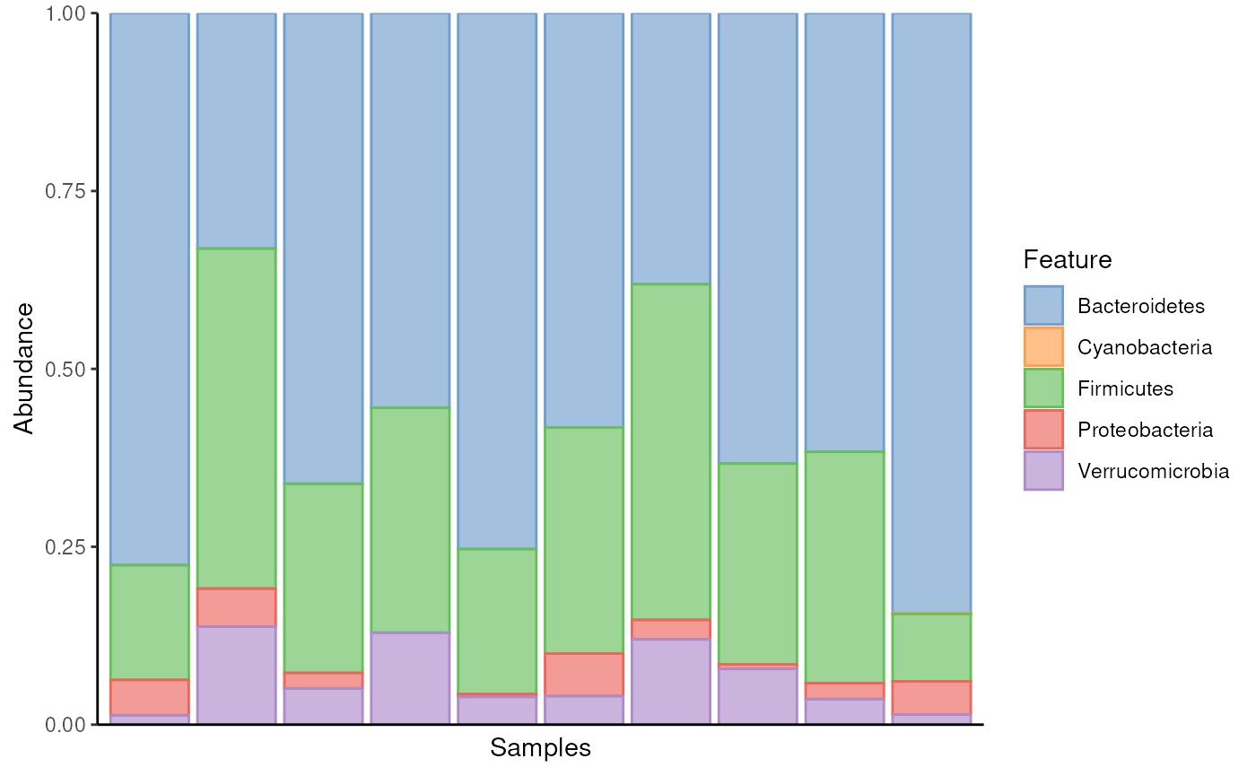
As we can see, Bacteroidetes is a common phylum in all samples. When its abundance drops below 50%, Firmicutes notably increases to fill the space.
Community diversity
Community diversity measures in microbiology can be categorized into three groups:
- Richness: The total number of taxonomic features.
- Equitability: How evenly the abundances of taxonmic features are distributed.
- Diversity: A combination of taxonomic feature richness and equitability.
Diversity can vary in association with different phenotypes. Next, we will calculate Faith’s phylogenetic diversity index. What sets this index apart is its incorporation of phylogeny into the diversity calculation. This index considers both the number and the relatedness of different taxonomic features, using branch lengths on a phylogenetic tree. For more information on diversity, see OMA.
# Estimate Faith's index
tse <- addAlpha(tse, index = "faith")
The results are stored to colData. The calculated index
shows how diverse each sample is in terms of the number of different
microbes present. We can then create a graph to visualize this.
p <- plotColData(tse, x = "patient_status", y = "faith")
p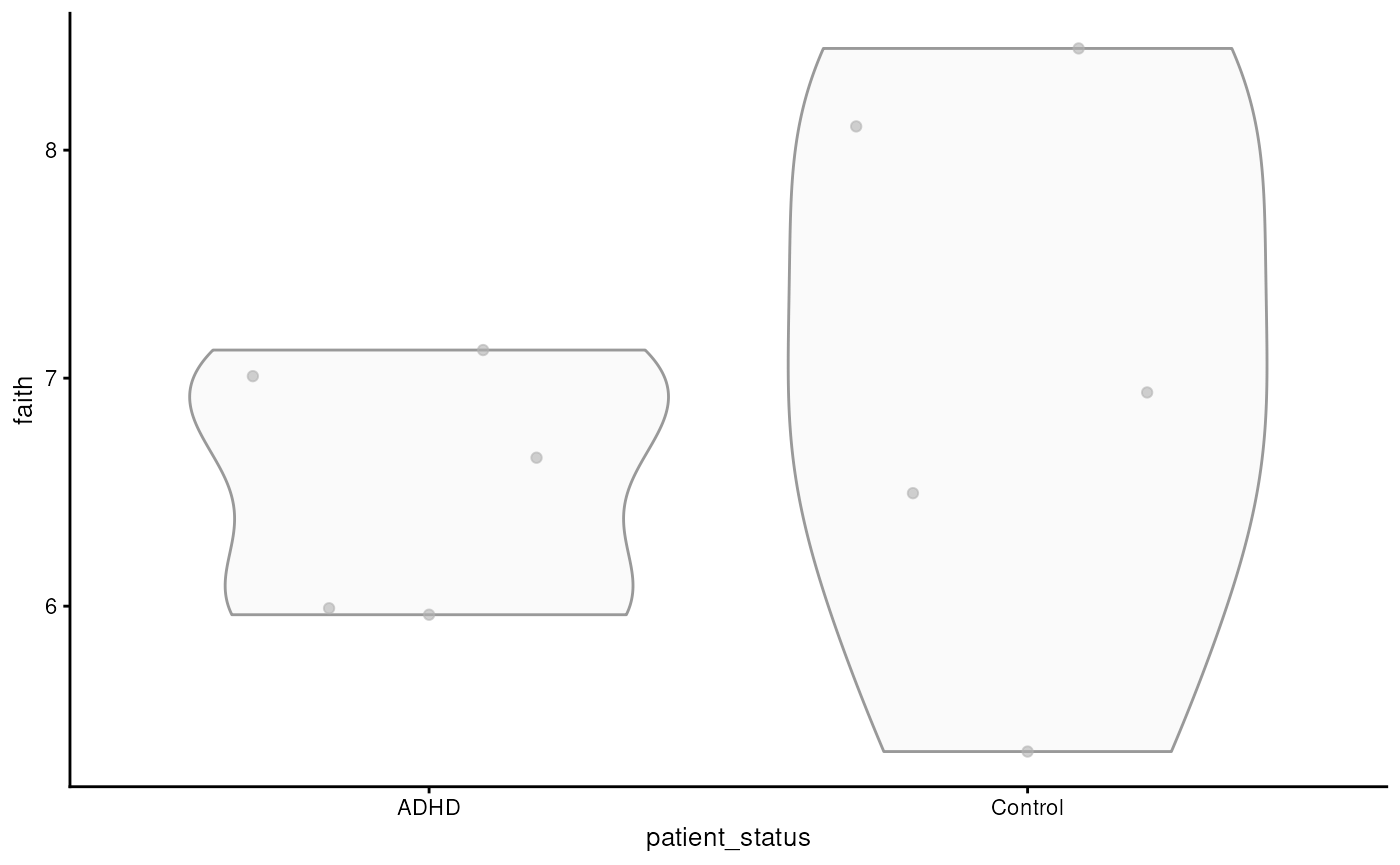
The graph shows that there is no significant difference in microbial diversity between the ADHD and control groups. However, alpha diversity metrics like Faith’s index only tell us about the diversity within individual samples and do not account for the differences between samples or groups. To understand how microbial communities vary between different samples — for instance, between ADHD patients and controls — we need to examine beta diversity.
Community dissimilarity
To gain a more comprehensive understanding of microbial variation across different samples, we assess beta diversity by measuring the dissimilarities in microbial compositions between samples. Beta diversity helps us determine how distinct or similar the microbiomes are among groups, allowing us to identify patterns or differences in microbial communities that may not be apparent from alpha diversity alone.
To explore these dissimilarities, we use Principal Coordinate Analysis (PCoA), a technique that reduces the complexity of high-dimensional data by projecting it into a lower-dimensional space while preserving the dissimilarities (or distances) between samples. This enables us to visualize the relationships and differences between samples in a simplified manner. For more information, refer to OMA.
In this analysis, we use UniFrac dissimilarity, which takes into account the phylogenetic relationships among features. UniFrac measures the phylogenetic distance between microbial communities by comparing the branch lengths shared by the communities on a phylogenetic tree. This provides a more nuanced understanding of community differences by incorporating evolutionary relationships.
# Run PCoA
tse <- addMDS(
    tse,
    FUN = getDissimilarity,
    tree = rowTree(tse),
    method = "unifrac",
    assay.type = "counts",
    niter = 100
    )
The results are stored in reducedDim slot. In order to
visualize this newly generated projection, we can apply
scater::plotReducedDim().
# Create a ggplot object
p <- plotReducedDim(
    tse, "MDS",
    colour_by = "patient_status",
    point_size = 3
    )
p <- p + labs(title = "Principal Coordinate Analysis")
p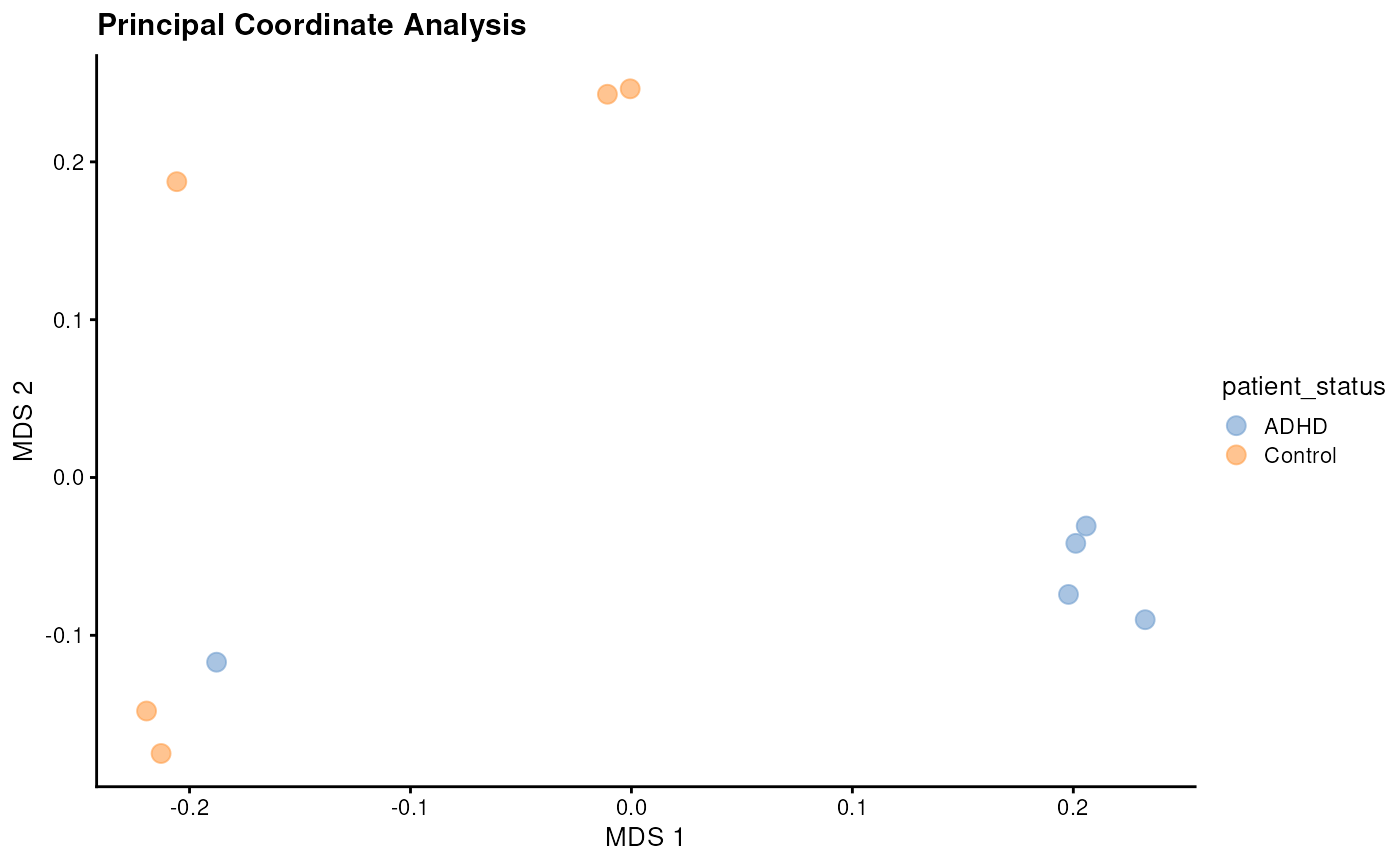
The plot shows that the data clusters into three groups, with two of them consisting solely of one diagnosis or another. This suggests that the microbial profiles differ between ADHD patients and controls.
To further explore the factors driving these differences in microbial profiles, we can perform a differential abundance analysis, for instance (see OMA).